Image from freepik 

 

Introduction

 

Support Vector Machine (SVM) is one of the most popular machine learning algorithms especially in the pre-boosting era (before the introduction of boosting algorithms), which is used for both Classification and Regression use-cases. 

The objective of an SVM classifier is to find the best n-1 dimensional hyperplane also called the decision boundary which can separate an n-dimensional space into the classes of interest. Notably, a hyperplane is a subspace whose dimension is one less than that of its ambient space.

SVM identifies the endpoints or end vectors that support this hyperplane while also maximizing the distance between them. This is the reason they are called support vectors, and thus the algorithm is called Support Vector Machines. 

The below diagram shows two classes segregated by a hyperplane:

 

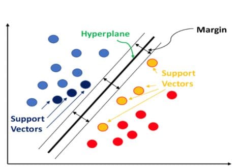
Source:https://datatron.com/wp-content/uploads/2021/05/Support-Vector-Machine.png

 

Why is SVM so popular?

 

When compared to simpler algorithms for example Logistic Regression, the SVM identification of maximum margin makes it a robust choice when dealing with noise. Particularly when a sample of one class crosses over to the other side across the decision boundary.

Logistic regression on the other hand is very vulnerable to such noisy samples and even a small sample of noisy observations can spoil the sport. The basic idea is that Logistic Regression is not trying to maximize the separation between the classes and just arbitrarily stops at a decision boundary that classifies the two categories correctly.

 

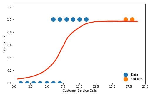
Source: https://kajabi-storefronts-production.kajabi-cdn.com/kajabi-storefronts-production/blogs/2147494064/images/N5bIuCEvQL6ZFNY3GCiX_LR3.png
 

Having a soft margin also allows for a budget for misclassifications and thus makes SVM robust to cross-overs across classes.

 

Source: https://vitalflux.com/wp-content/uploads/2015/03/logistic-regression-vs-SVM.png
 

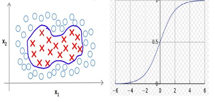
Kernel functions are another reason why SVM is so popular. SVM classifier is able to separate the classes with non-linear decision boundaries.

We will discuss more on Soft margin and Kernel Trick in the upcoming sections, but let us first put focus on the precursor to soft margin i.e. hard margin SVM.

 

Hard Margin SVM

 

Let's start our discussion with a straightforward and relatively easier-to-understand version of SVM called Hard Margin SVM or just Maximal Margin Classifier.

The perpendicular distance between the two support vectors when the two classes of interest are linearly separable is called a margin. The only thing to observe here is that the two classes are distinctly positioned with respect to each other which means not even a single sample crosses over across the margin.

Let's go a little deeper into the mathematics of a Hard Margin Support Vector Machine.

In the diagram below, we have a positive class denoted by green and a negative denoted by red. Now to maximize the margin or the distance between the two classes we need to assume a perpendicular vector to our decision boundary. 

 

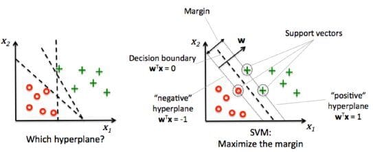
Source: https://qph.cf2.quoracdn.net/main-qimg-8264205dc003f4e1c15a3d060b9375ee-pjlq
 

Under the following constraints:

 

 

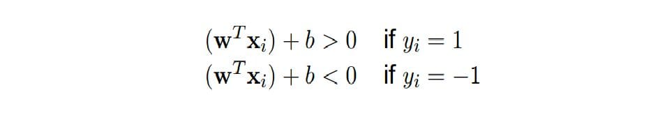
This is because the samples to the right of the margin should be classified as positive and to the left of the margin should be classified as negative.

We can also write the objective function as:

 

 

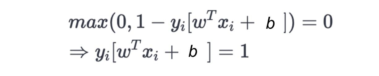
This is called Hinge Loss, which takes care of the correct classification of the two classes.

 

Soft Margin SVM

 

Real-world data does not follow the ideal assumption of linear separability as in the case with Hard Margin. The solution is to allow a tiny misclassification or violation of the margin in such a way that the overall margin is maximized. The Maximal Margin Classifier that uses a soft margin instead of a hard margin is called a Soft Margin Classifier.

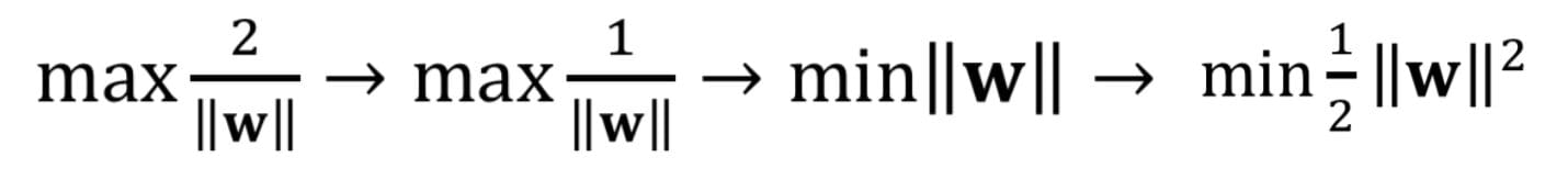
Let the perpendicular vector be “w” and our objective is to maximize the number of steps in either direction from the decision boundary assuming it's in the middle of both support vectors. Solving the above equation would give us the margin as below:

Maximizing the above quantity alternatively means minimizing ||w|| or square of that, and in turn maximizing the margin of the classifier.

 

 

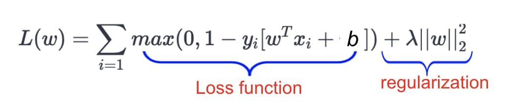
This allows an additional term to the hinge loss equation discussed in the hard margin case where the ||w||² terms make sure that the model balances correct classification with maximizing the margin. The equation given below shows the two components of a soft margin SVM where the second term acts as a regularize.

 

Source: https://miro.medium.com/max/1042/1*nFmhvEy6GyYQOYlF-L9XRw.png
 

Here lambda is a hyperparameter and can be tuned to allow more or fewer misclassifications. A higher value of lambda means a higher allowance of misclassifications whereas a lower value of lambda restricts misclassifications to a minimum.

 

Kernel Trick

 

The world is not ideal and thus not all classification problems have linearly separable classes. Kernel Functions in SVM allow us to solve such cases.

Below is an example of how a polynomial kernel function (degree 2 polynomial) is applied to a non-linear separable case to make it linear separable.

 

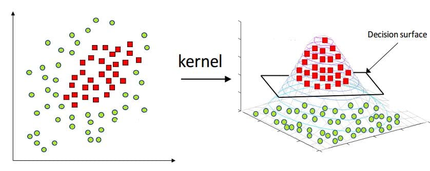
Source: https://miro.medium.com/max/1400/1*mCwnu5kXot6buL7jeIafqQ.png
 

Some of the popular kernels are listed below:

 

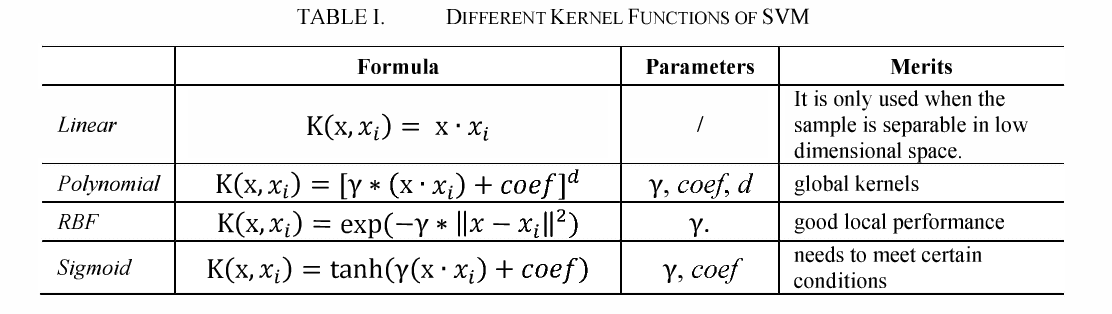
Source: https://d3i71xaburhd42.cloudfront.net/3a92a26a66efba1849fa95c900114b9d129467ac/3-TableI-1.png
 

Kernels are amazing as they let you project the data in an additional dimension without adding an overhead of a dimension.

 

Summary

 

We discussed the significance of the SVM classifier and its application especially when the number of dimensions is very high as compared to the number of examples. This makes it really effective in NLP problems where a lot of times text is converted to really long vectors of numbers. Further, we learnt about the kernel functions which aid its ability to classify the new data points across non-linear decision boundaries. Besides, SVM models are immune to overfitting to a large extent as the decision boundary is only affected by support vectors and is largely immune to the presence of the other extreme observations. 

 
 
Vidhi Chugh is an award-winning AI/ML innovation leader and an AI Ethicist. She works at the intersection of data science, product, and research to deliver business value and insights. She is an advocate for data-centric science and a leading expert in data governance with a vision to build trustworthy AI solutions.