Machine Learning: What is Bootstrapping?
Bootstrapping is an essential technique if you're into machine learning. We’ll discuss it from theoretical and practical standpoints. The practical part involves two examples of bootstrapping in Python.

Image by Author
Machine learning is a growing field that is transforming the way we process and analyze data.
Bootstrapping is an important technique in the world of machine learning. It is crucial for building robust and accurate models.
In this article, we will dive into what bootstrapping is and how it can be used in machine learning.
Also, we will explore the decision tree classifier and the Iris data set. It will be used to show bootstrapping in a real-world example.
Through this article, we aim to provide a comprehensive understanding of bootstrapping.
Also, we will cover its applications in machine learning. That will equip you with the knowledge to apply it to your own machine learning projects.
But first, what is bootstrapping?
What is Bootstrapping?
Bootstrapping is a resampling technique that helps in estimating the uncertainty of a statistical model.
It includes sampling the original dataset with replacement and generating multiple new datasets of the same size as the original.
Each of these new datasets is then used to calculate the desired statistic, such as the mean or standard deviation.
This process is repeated multiple times, and the resulting values are used to construct a probability distribution for the desired statistic.
This technique is often used in machine learning to estimate the accuracy of a model, validate its performance, and identify areas that need improvement.
For example, we can use bootstrap sampling to calculate the population means. Also, the result would be as follows.
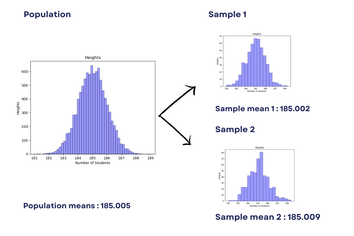
Image by Author
We also will cover this example later in this article.
How to Use Bootstrapping in Machine Learning?
Bootstrapping can be used in machine learning in several ways, including the estimation of model performance, model selection, and identifying the most important features in a dataset.
One of the popular use cases of bootstrapping in machine learning is to estimate the accuracy of a classifier, which we will do in this article.
Let’s start with an easy example of bootstrapping in Python as a warmup.
Bootstrapping in Calculating Mean
We will show how bootstrapping can be used to estimate the mean height of students in a school of 10,000 students.
The general approach is to calculate the mean by summing up all heights and dividing the sum by 10,000.
First, generate a sample of 10,000 randomly generated numbers (heights) using the NumPy library.
import numpy as np
import pandas as pd
x = np.random.normal(loc= 185.0, scale=1.0, size=10000)
np.mean(x)
Here is the output of the mean.
Now, how can we calculate the height of these students just from 200 students?
In bootstrap sampling, we create several samples of the population by randomly selecting elements from the population with replacements.
In our example, the sample size will be 5. It means there will be 40 samples for the population of 200 students.
With the code below, we will draw 40 samples, size of 5, from the students. (x)
This involves drawing random samples with replacements from the original sample to create 40 new samples.
What do I mean by replacements?
I mean first selecting one of 10,000, forgetting who I chose, then selecting one of 10,000 again.
You can select the same student, but there is a small chance of that. Replacements don’t sound that clever anymore, right?
Each new sample has a size of 5, which is smaller than the original sample. The mean of each new sample is calculated and stored in the sample_mean list.
Finally, the mean of all 40 sample means is calculated and represents the estimate of the population mean.
Here is the code.
import random

sample_mean = []

# Bootstrap Sampling
for i in range(40):
    y = random.sample(x.tolist(), 5)
    avg = np.mean(y)

    sample_mean.append(avg)
np.mean(sample_mean)
Here is the output.
It is pretty close, right?
Bootstrapping in Classification Task With a Decision Tree
Here, we will see the usage of bootstrapping in classification with a decision tree by using the Iris data set. But first, let’s see what a decision tree is.
What Is a Decision Tree?
A decision tree is one of the popular machine learning algorithms that is widely used for both classification and regression problems. It is a tree-based model that involves making predictions by branching out from the root node and making decisions based on certain conditions.
The decision tree classifier is a specific implementation of this algorithm used to perform binary classification tasks.
The main goal of the decision tree classifier is to determine the most important features that contribute to the prediction of a target variable. The algorithm uses a greedy approach to minimize the impurity of the tree by selecting the feature with the highest information gain. The tree continues to split until the data is completely pure or until a stopping criterion is reached.
What Is the Iris Data Set?
The Iris data set is one of the popular data sets used to evaluate classification tasks.
This data set contains 150 observations of iris flowers, where each observation contains the features such as sepal length, sepal width, petal length, and petal width.
The target variable is the species of the iris plant.
The Iris data set is widely used in machine learning algorithms to evaluate the performance of different models and is also used as an example to demonstrate the concept of decision tree classifiers.
Let’s now see how to use bootstrapping and a decision tree in classification.
Coding of Bootstrapping
The code implements a bootstrapping technique for a machine learning model using the DecisionTreeClassifier from the sci-kit-learn library.
The first few lines load the Iris dataset and extract the feature data (X) and target data (y) from it.
The bootstrap function takes in the feature data (X), target data (y), and the number of samples (n_samples) to use in bootstrapping.
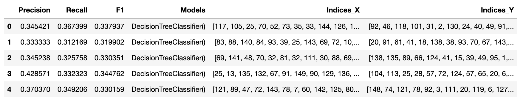
The function returns a list of trained models and a pandas data frame with precision, recall, F1 score, and the indices used for bootstrapping.
The bootstrapping process is done in a for loop.
For each iteration, the function uses the np.random.choice method to randomly select a sample of the feature data (X) and target data (y).
The sample data is then split into training and testing sets using the train_test_split method. The DecisionTreeClassifier is trained on the training data and then used to make predictions on the testing data.
The precision, recall, and F1 scores are calculated using the metrics.precision_score, metrics.recall_score, and metrics.f1_score methods from the sci-kit-learn library. These scores are then added to a list for each iteration.
Finally, the results are saved to a pandas data frame with columns for precision, recall, F1 score, the trained models, and the indices used for bootstrapping. The data frame is then returned by the function.
Now, let's see the code.
from sklearn import metrics
import pandas as pd
from sklearn.model_selection import train_test_split
from sklearn.datasets import load_iris
from sklearn.tree import DecisionTreeClassifier

# Load the iris dataset
iris = load_iris()
X, y = iris.data, iris.target


def bootstrap(X, y, n_samples=2000):
    models = []
    precision = []
    recall = []
    f1 = []
    indices_x = []
    indices_y = []

    for i in range(n_samples):
        index_x = np.random.choice(X.shape[0], size=X.shape[0], replace=True)
        indices_x.append(index_x)
        X_sample = X[index_x, :]

        index_y = np.random.choice(y.shape[0], size=y.shape[0], replace=True)
        indices_y.append(index_y)
        y_sample = y[index_y]

        X_train, X_test, y_train, y_test = train_test_split(
            X_sample, y_sample, test_size=0.2, random_state=42
        )

        model = DecisionTreeClassifier().fit(X_train, y_train)
        models.append(model)

        y_pred = model.predict(X_test)
        precision.append(
            metrics.precision_score(y_test, y_pred, average="macro")
        )
        recall.append(metrics.recall_score(y_test, y_pred, average="macro"))
        f1.append(metrics.f1_score(y_test, y_pred, average="macro"))
    # Save the results to a Pandas dataframe
    pred_df = pd.DataFrame(
        {
            "Precision": precision,
            "Recall": recall,
            "F1": f1,
            "Models": models,
            "Indices_X": indices_x,
            "Indices_Y": indices_y,
        }
    )
Now call the function.
models, pred_df = bootstrap(X, y)
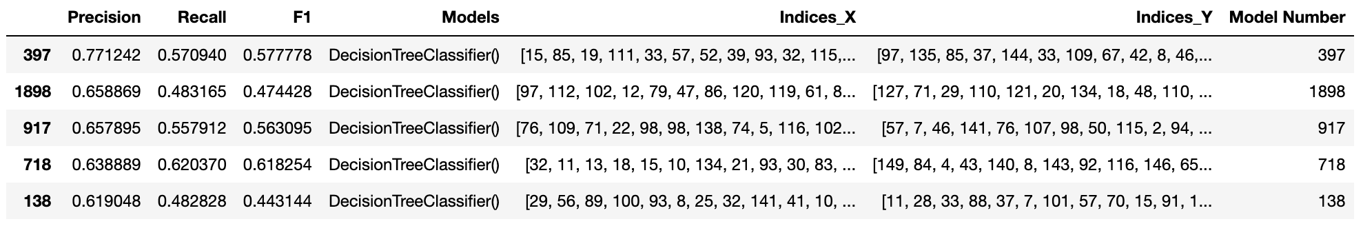
Show the results of the data frame that the function creates.
pred_df.head()
Now add the index column as the model number,
pred_df['Model Number'] = pred_df.index,
and sort the values by precision.
pred_df.sort_values(by= "Precision", ascending = False).head(5)
To see the results better, we will make some data visualization.
Bootstrapping Visualization
The code below creates 3 bar graphs to show the performance of bootstrapped models.
The performance of the models is measured by the precision, recall, and F1 scores. So, we will create a data frame called pred_df. This data frame stores the scores of the models.
The code creates a figure with 3 subplots.
The first subplot (ax2) is a bar graph that shows the precision scores of the top 5 models.
The x-axis shows the precision score, and the y-axis shows the model's index. For each bar, the value is displayed in the center of these 3 figures. The title of this graph is "Precision".
The second subplot (ax3) is a bar graph that shows the recall scores of the top 5 models. The x-axis shows the recall score, and the y-axis shows the model's index. The title of this graph is "Recall".
The third subplot (ax4) is a bar graph that shows the F1 scores of the top 5 models. The x-axis shows the F1 score, and the y-axis shows the model's index. The title of this graph is "F1".
The overall title of the figure is "Bootstrapped Model Performance Metrics". We will display these images by using plt.show().
Here is the code.
import matplotlib.pyplot as plt

# Create a figure and subplots
fig, (ax2, ax3, ax4) = plt.subplots(1, 3, figsize=(14, 8))

best_of = pred_df.sort_values(by="Precision", ascending=False).head(5)

# Create the first graph
best_of.plot(
    kind="barh",
    x="Model Number",
    y="Precision",
    color="mediumturquoise",
    ax=ax2,
    legend=False,
)
ax2.set_xlabel(
    "Precision Score",
    fontstyle="italic",
    fontsize=14,
    font="Courier New",
    fontweight="bold",
    y=1.1,
)
ylabel = "Model\nName"
ax2.set_ylabel(ylabel, fontsize=16, font="Courier")
ax2.set_title("Precision", fontsize=16, fontstyle="italic")


for index, value in enumerate(best_of["Precision"]):
    ax2.text(
        value / 2,
        index,
        str(round(value, 2)),
        ha="center",
        va="center",
        fontsize=14,
        font="Comic Sans MS",
    )
best_of = pred_df.sort_values(by="Recall", ascending=False).head(5)

# Create the second graph
best_of.plot(
    kind="barh",
    x="Model Number",
    y="Recall",
    color="orange",
    ax=ax3,
    legend=False,
)
ax3.set_xlabel(
    "Recall Score",
    fontstyle="italic",
    fontsize=14,
    font="Courier New",
    fontweight="bold",
)
ax3.set_ylabel(ylabel, fontsize=16, font="Courier")
ax3.set_title("Recall", fontsize=16, fontstyle="italic")

for index, value in enumerate(best_of["Recall"]):
    ax3.text(
        value / 2,
        index,
        str(round(value, 2)),
        ha="center",
        va="center",
        fontsize=14,
        font="Comic Sans MS",
    )
# Create the third graph
best_of = pred_df.sort_values(by="F1", ascending=False).head(5)
best_of.plot(
    kind="barh",
    x="Model Number",
    y="F1",
    color="darkorange",
    ax=ax4,
    legend=False,
)
ax4.set_xlabel(
    "F1 Score",
    fontstyle="italic",
    fontsize=14,
    font="Courier New",
    fontweight="bold",
)
ax4.set_ylabel(ylabel, fontsize=16, font="Courier")
ax4.set_title("F1", fontsize=16, fontstyle="italic")


for index, value in enumerate(best_of["F1"]):
    ax4.text(
        value / 2,
        index,
        str(round(value, 2)),
        ha="center",
        va="center",
        fontsize=14,
        font="Comic Sans MS",
    )
# Fit the figure
plt.tight_layout()

plt.suptitle(
    "Bootstrapped Model Performance Metrics",
    fontsize=18,
    y=1.05,
    fontweight="bold",
    fontname="Comic Sans MS",
)

# Show the figure
plt.show()
Here is the output.
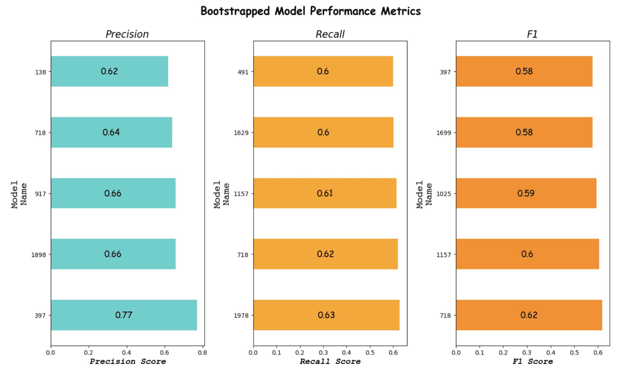
Image by Author
It looks like Model 397 is our best model according to the precision and F1 score.
Of course, if the recall is more important for your project, you can choose Model 718 or another.
Reproducing Best Results
Now, we have already saved the indices to create reproducible results. We will select the 397th model and see the results whether the results are reproducible or not.
The following code starts by selecting a sample of the data (X and y) using the indices stored in the 397th row of the pred_df data frame.
The sample data is then split into training and testing datasets using the train_test_split method with a test size of 0.2 and a random state of 42.
Next, a decision tree classifier model is trained using the training data and stored in the model's list. The trained model is then used to make predictions on the test data using the predict() method.
Finally, the precision, recall, and F1 scores of the model are calculated using the precision_score, recall_score, and f1_score functions from the metrics module and printed to the console.
These scores evaluate the model's performance by measuring the model's ability to correctly classify the data and the level of false positives and false negatives generated by the model.
Here is the code.
X_sample = X[pred_df.iloc[397]["Indices_X"], :]
y_sample = y[pred_df.iloc[397]["Indices_Y"]]

X_train, X_test, y_train, y_test = train_test_split(
    X_sample, y_sample, test_size=0.2, random_state=42
)

model = DecisionTreeClassifier().fit(X_train, y_train)
models.append(model)

y_pred = model.predict(X_test)
precision_397 = metrics.precision_score(y_test, y_pred, average="macro")
recall_397 = metrics.recall_score(y_test, y_pred, average="macro")
f1_397 = metrics.f1_score(y_test, y_pred, average="macro")
print("Precision : {}".format(precision_397))
print("Recall : {}".format(recall_397))
print("F1 : {}".format(f1_397))
Here is the output.

Conclusion
In conclusion, bootstrapping is a powerful tool in machine learning that can be used to improve the performance of algorithms. By creating multiple subsets of the data, bootstrapping helps to reduce the risk of overfitting and improves the accuracy of the results.
We demonstrated how to use bootstrapping for the classification algorithm with a decision tree classifier.
By combining bootstrapping and decision tree classifier, we can create a powerful machine learning model that provides accurate and reliable results, which might be applied to other classification algorithms.
Understanding all the mentioned concepts is essential for data scientists and machine learning professionals. Mandatory, I would say! They allow you to make informed decisions about the tools and techniques they use to solve real-world problems.
Nate Rosidi is a data scientist and in product strategy. He's also an adjunct professor teaching analytics, and is the founder of StrataScratch, a platform helping data scientists prepare for their interviews with real interview questions from top companies. Connect with him on Twitter: StrataScratch or LinkedIn.