Multi-label NLP: An Analysis of Class Imbalance and Loss Function Approaches
In this comprehensive article, we have demonstrated that a seemingly simple task of multi-label text classification can be challenging when traditional methods are applied. We have proposed the use of distribution-balancing loss functions to tackle the issue of class imbalance.
Multi-label NLP refers to the task of assigning multiple labels to a given text input, rather than just one label. In traditional NLP tasks, such as text classification or sentiment analysis, each input is typically assigned a single label based on its content. However, in many real-world scenarios, a piece of text can belong to multiple categories or express multiple sentiments simultaneously.
Multi-label NLP is important because it allows us to capture more nuanced and complex information from text data. For example, in the domain of customer feedback analysis, a customer review may express both positive and negative sentiments at the same time, or it may touch upon multiple aspects of a product or service. By assigning multiple labels to such inputs, we can gain a more comprehensive understanding of the customer's feedback and take more targeted actions to address their concerns.
This article delves into a noteworthy case of Provectus’ use of multi-label NLP.
Context:
A client approached us with a request to help them automate labeling documents of a certain type. At first glance, the task appeared to be straightforward and easily solved. However, as we worked on the case, we encountered a dataset with inconsistent annotations. Though our customer had faced challenges with varying class numbers and changes in their review team over time, they had invested significant efforts into creating a diverse dataset with a range of annotations. While there existed some imbalances and uncertainties in the labels, this dataset provided a valuable opportunity for analysis and further exploration.
Let’s take a closer look at the dataset, explore the metrics and our approach, and recap how Provectus solved the problem of multi-label text classification.
Overview of the Dataset
The dataset has 14,354 observations, with 124 unique classes (labels). Our task is to assign one or multiple classes to every observation.
Table 1 provides descriptive statistics for the dataset.
On average, we have about two classes per observation, with an average of 261 different texts describing a single class.
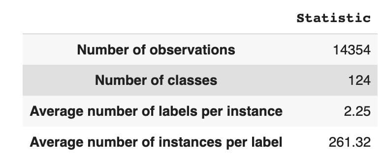
Table 1: Dataset Statistic
In Figure 1, we see the distribution of classes in the top graph, and we have a certain number of HEAD labels with the highest frequency of occurrence in the dataset. Also note that the majority of classes have a low frequency of occurrence.
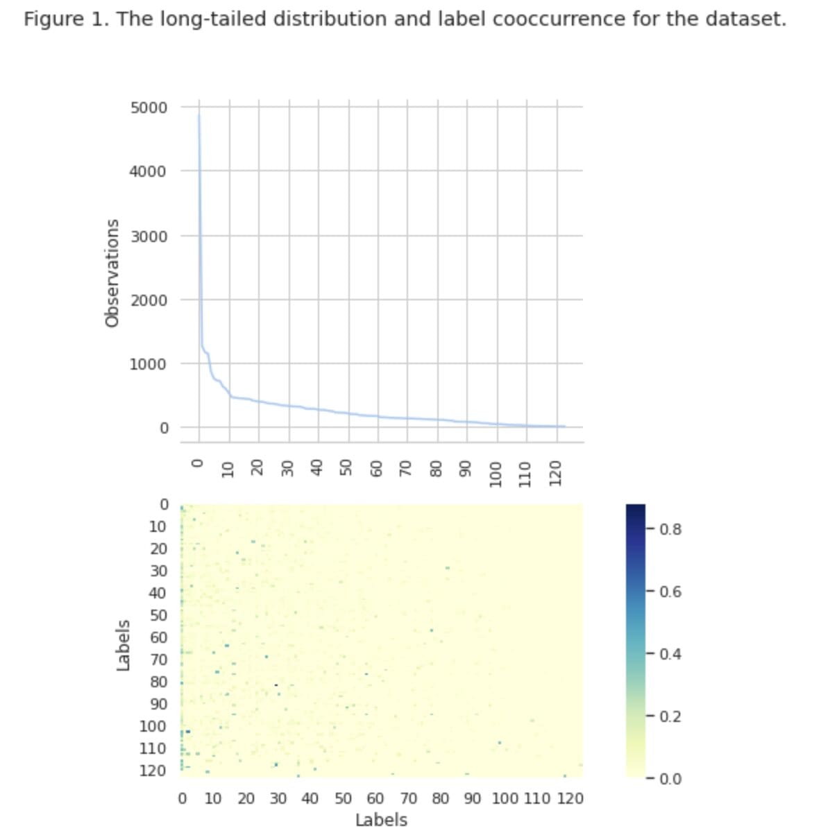
In the bottom graph we see that there is frequent overlap between the classes that are best represented in the dataset, and the classes that have low significance.
We changed the process of splitting the dataset into train/val/test sets. Instead of using a traditional method, we have employed iterative stratification, to provide a well-balanced distribution of evidence of label relations. For that, we used Scikit Multi-learn
from skmultilearn.model_selection import iterative_train_test_split

mlb = MultiLabelBinarizer()


def balanced_split(df, mlb, test_size=0.5):
    ind = np.expand_dims(np.arange(len(df)), axis=1)
    mlb.fit_transform(df["tag"])
    labels = mlb.transform(df["tag"])
    ind_train, _, ind_test, _ = iterative_train_test_split(
        ind, labels, test_size
    )
    return df.iloc[ind_train[:, 0]], df.iloc[ind_test[:, 0]]


df_train, df_tmp = balanced_split(df, test_size=0.4)
df_val, df_test = balanced_split(df_tmp, test_size=0.5)
We obtained the following distribution:
- The training dataset contains 60% of the data and covers all 124 labels
- The validation dataset contains 20% of the data and covers all 124 labels
- The test dataset contains 20% of the data and covers all 124 labels
Metrics Applied
Multi-label classification is a type of supervised machine learning algorithm that allows us to assign multiple labels to a single data sample. It differs from binary classification where the model predicts only two categories, and multi-class classification where the model predicts only one out of multiple classes for a sample.
Evaluation metrics for multi-label classification performance are inherently different from those used in multi-class (or binary) classification due to the inherent differences of the classification problem. More detailed information can be found on Wikipedia.
We selected metrics that are most suitable for us:
- Precision measures the proportion of true positive predictions among the total positive predictions made by the model.
- Recall measures the proportion of true positive predictions among all actual positive samples.
- F1-score is the harmonic mean of precision and recall, which helps to restore balance between the two.
- Hamming loss is the fraction of labels that are incorrectly predicted
We also track the number of predicted labels in the set { defined as count for labels, for which we achieve an F1 score > 0}.
K. I. S. S. Approach
Multi-Label Classification is a type of supervised learning problem where a single instance or example can be associated with multiple labels or classifications, as opposed to traditional single-label classification, where each instance is only associated with a single class label.
To solve multi-label classification problems, there are two main categories of techniques:
- Problem transformation methods
- Algorithm adaptation methods
Problem transformation methods enable us to transform multi-label classification tasks into multiple single-label classification tasks. For example, the Binary Relevance (BR) baseline approach treats every label as a separate binary classification problem. In this case, the multi-label problem is transformed into multiple single-label problems.
Algorithm adaptation methods modify the algorithms themselves to handle multi-label data natively, without transforming the task into multiple single-label classification tasks. An example of this approach is the BERT model, which is a pre-trained transformer-based language model that can be fine-tuned for various NLP tasks, including multi-label text classification. BERT is designed to handle multi-label data directly, without the need for problem transformation.
In the context of using BERT for multi-label text classification, the standard approach is to use Binary Cross-Entropy (BCE) loss as the loss function. BCE loss is a commonly used loss function for binary classification problems and can be easily extended to handle multi-label classification problems by computing the loss for each label independently, and then summing the losses. In this case, the BCE loss function measures the error between predicted probabilities and true labels, where predicted probabilities are obtained from the final sigmoid activation layer in the BERT model.
Now, let's take a closer look at Figure 2 below.
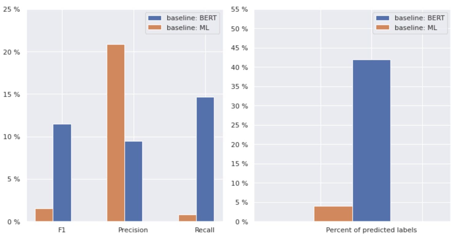
Figure 2. Metrics for baseline models
The graph on the left shows a comparison of metrics for a “baseline: BERT” and “baseline: ML”. Thus, it can be seen that for “baseline: BERT”, the F1 and Recall scores are approximately 1.5 times higher, while the Precision for “baseline: ML” is 2 times higher than that of model 1. By analyzing the overall percentage of predicted classes shown on the right, we see that “baseline: BERT” predicted classes more than 10 times that of “baseline: ML”.
Because the maximum result for the “baseline: BERT” is less than 50% of all classes, the results are quite discouraging. Let’s figure out how to improve these results.
Golden Ratio of Approaches
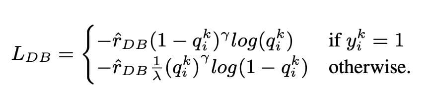
Based on the outstanding article "Balancing Methods for Multi-label Text Classification with Long-Tailed Class Distribution", we learned that distribution-balanced loss may be the most suitable approach for us.
Distribution-balanced loss
Distribution-balanced loss is a technique used in multi-label text classification problems to address imbalances in class distribution. In these problems, some classes have a much higher frequency of occurrence compared to others, resulting in model bias toward these more frequent classes.
To address this issue, distribution-balanced loss aims to balance the contribution of each sample in the loss function. This is achieved by re-weighting the loss of each sample based on the inverse of its frequency of occurrence in the dataset. By doing so, the contribution of less frequent classes is increased, and the contribution of more frequent classes is decreased, thus balancing the overall class distribution.
This technique has been shown to be effective in improving the performance of models on long-tailed class distribution problems. By reducing the impact of frequent classes and increasing the impact of infrequent classes, the model is able to better capture patterns in the data and produce more balanced predictions.
Implementation of Resample Class
import torch
import torch.nn as nn
import torch.nn.functional as F
import numpy as np


class ResampleLoss(nn.Module):
    def __init__(
        self,
        use_sigmoid=True,
        partial=False,
        loss_weight=1.0,
        reduction="mean",
        reweight_func=None,
        weight_norm=None,
        focal=dict(focal=True, alpha=0.5, gamma=2),
        map_param=dict(alpha=10.0, beta=0.2, gamma=0.1),
        CB_loss=dict(CB_beta=0.9, CB_mode="average_w"),
        logit_reg=dict(neg_scale=5.0, init_bias=0.1),
        class_freq=None,
        train_num=None,
    ):
        super(ResampleLoss, self).__init__()
        assert (use_sigmoid is True) or (partial is False)
        self.use_sigmoid = use_sigmoid
        self.partial = partial
        self.loss_weight = loss_weight
        self.reduction = reduction
        if self.use_sigmoid:
            if self.partial:
                self.cls_criterion = partial_cross_entropy
            else:
                self.cls_criterion = binary_cross_entropy
        else:
            self.cls_criterion = cross_entropy
        # reweighting function
        self.reweight_func = reweight_func
        # normalization (optional)
        self.weight_norm = weight_norm
        # focal loss params
        self.focal = focal["focal"]
        self.gamma = focal["gamma"]
        self.alpha = focal["alpha"]
        # mapping function params
        self.map_alpha = map_param["alpha"]
        self.map_beta = map_param["beta"]
        self.map_gamma = map_param["gamma"]
        # CB loss params (optional)
        self.CB_beta = CB_loss["CB_beta"]
        self.CB_mode = CB_loss["CB_mode"]
        self.class_freq = (
            torch.from_numpy(np.asarray(class_freq)).float().cuda()
        )
        self.num_classes = self.class_freq.shape[0]
        self.train_num = train_num  # only used to be divided by class_freq
        # regularization params
        self.logit_reg = logit_reg
        self.neg_scale = (
            logit_reg["neg_scale"] if "neg_scale" in logit_reg else 1.0
        )
        init_bias = (
            logit_reg["init_bias"] if "init_bias" in logit_reg else 0.0
        )
        self.init_bias = (
            -torch.log(self.train_num / self.class_freq - 1) * init_bias
        )
        self.freq_inv = (
            torch.ones(self.class_freq.shape).cuda() / self.class_freq
        )
        self.propotion_inv = self.train_num / self.class_freq

    def forward(
        self,
        cls_score,
        label,
        weight=None,
        avg_factor=None,
        reduction_override=None,
        **kwargs
    ):
        assert reduction_override in (None, "none", "mean", "sum")
        reduction = (
            reduction_override if reduction_override else self.reduction
        )
        weight = self.reweight_functions(label)
        cls_score, weight = self.logit_reg_functions(
            label.float(), cls_score, weight
        )
        if self.focal:
            logpt = self.cls_criterion(
                cls_score.clone(),
                label,
                weight=None,
                reduction="none",
                avg_factor=avg_factor,
            )
            # pt is sigmoid(logit) for pos or sigmoid(-logit) for neg
            pt = torch.exp(-logpt)
            wtloss = self.cls_criterion(
                cls_score, label.float(), weight=weight, reduction="none"
            )
            alpha_t = torch.where(label == 1, self.alpha, 1 - self.alpha)
            loss = alpha_t * ((1 - pt) ** self.gamma) * wtloss
            loss = reduce_loss(loss, reduction)
        else:
            loss = self.cls_criterion(
                cls_score, label.float(), weight, reduction=reduction
            )
        loss = self.loss_weight * loss
        return loss

    def reweight_functions(self, label):
        if self.reweight_func is None:
            return None
        elif self.reweight_func in ["inv", "sqrt_inv"]:
            weight = self.RW_weight(label.float())
        elif self.reweight_func in "rebalance":
            weight = self.rebalance_weight(label.float())
        elif self.reweight_func in "CB":
            weight = self.CB_weight(label.float())
        else:
            return None
        if self.weight_norm is not None:
            if "by_instance" in self.weight_norm:
                max_by_instance, _ = torch.max(weight, dim=-1, keepdim=True)
                weight = weight / max_by_instance
            elif "by_batch" in self.weight_norm:
                weight = weight / torch.max(weight)
        return weight

    def logit_reg_functions(self, labels, logits, weight=None):
        if not self.logit_reg:
            return logits, weight
        if "init_bias" in self.logit_reg:
            logits += self.init_bias
        if "neg_scale" in self.logit_reg:
            logits = logits * (1 - labels) * self.neg_scale + logits * labels
            if weight is not None:
                weight = (
                    weight / self.neg_scale * (1 - labels) + weight * labels
                )
        return logits, weight

    def rebalance_weight(self, gt_labels):
        repeat_rate = torch.sum(
            gt_labels.float() * self.freq_inv, dim=1, keepdim=True
        )
        pos_weight = (
            self.freq_inv.clone().detach().unsqueeze(0) / repeat_rate
        )
        # pos and neg are equally treated
        weight = (
            torch.sigmoid(self.map_beta * (pos_weight - self.map_gamma))
            + self.map_alpha
        )
        return weight

    def CB_weight(self, gt_labels):
        if "by_class" in self.CB_mode:
            weight = (
                torch.tensor((1 - self.CB_beta)).cuda()
                / (1 - torch.pow(self.CB_beta, self.class_freq)).cuda()
            )
        elif "average_n" in self.CB_mode:
            avg_n = torch.sum(
                gt_labels * self.class_freq, dim=1, keepdim=True
            ) / torch.sum(gt_labels, dim=1, keepdim=True)
            weight = (
                torch.tensor((1 - self.CB_beta)).cuda()
                / (1 - torch.pow(self.CB_beta, avg_n)).cuda()
            )
        elif "average_w" in self.CB_mode:
            weight_ = (
                torch.tensor((1 - self.CB_beta)).cuda()
                / (1 - torch.pow(self.CB_beta, self.class_freq)).cuda()
            )
            weight = torch.sum(
                gt_labels * weight_, dim=1, keepdim=True
            ) / torch.sum(gt_labels, dim=1, keepdim=True)
        elif "min_n" in self.CB_mode:
            min_n, _ = torch.min(
                gt_labels * self.class_freq + (1 - gt_labels) * 100000,
                dim=1,
                keepdim=True,
            )
            weight = (
                torch.tensor((1 - self.CB_beta)).cuda()
                / (1 - torch.pow(self.CB_beta, min_n)).cuda()
            )
        else:
            raise NameError
        return weight

    def RW_weight(self, gt_labels, by_class=True):
        if "sqrt" in self.reweight_func:
            weight = torch.sqrt(self.propotion_inv)
        else:
            weight = self.propotion_inv
        if not by_class:
            sum_ = torch.sum(weight * gt_labels, dim=1, keepdim=True)
            weight = sum_ / torch.sum(gt_labels, dim=1, keepdim=True)
        return weight


def reduce_loss(loss, reduction):
    """Reduce loss as specified.
    Args:
        loss (Tensor): Elementwise loss tensor.
        reduction (str): Options are "none", "mean" and "sum".
    Return:
        Tensor: Reduced loss tensor.
    """
    reduction_enum = F._Reduction.get_enum(reduction)
    # none: 0, elementwise_mean:1, sum: 2
    if reduction_enum == 0:
        return loss
    elif reduction_enum == 1:
        return loss.mean()
    elif reduction_enum == 2:
        return loss.sum()


def weight_reduce_loss(loss, weight=None, reduction="mean", avg_factor=None):
    """Apply element-wise weight and reduce loss.
    Args:
        loss (Tensor): Element-wise loss.
        weight (Tensor): Element-wise weights.
        reduction (str): Same as built-in losses of PyTorch.
        avg_factor (float): Avarage factor when computing the mean of losses.
    Returns:
        Tensor: Processed loss values.
    """
    # if weight is specified, apply element-wise weight
    if weight is not None:
        loss = loss * weight
    # if avg_factor is not specified, just reduce the loss
    if avg_factor is None:
        loss = reduce_loss(loss, reduction)
    else:
        # if reduction is mean, then average the loss by avg_factor
        if reduction == "mean":
            loss = loss.sum() / avg_factor
        # if reduction is 'none', then do nothing, otherwise raise an error
        elif reduction != "none":
            raise ValueError(
                'avg_factor can not be used with reduction="sum"'
            )
    return loss


def binary_cross_entropy(
    pred, label, weight=None, reduction="mean", avg_factor=None
):
    # weighted element-wise losses
    if weight is not None:
        weight = weight.float()
    loss = F.binary_cross_entropy_with_logits(
        pred, label.float(), weight, reduction="none"
    )
    loss = weight_reduce_loss(
        loss, reduction=reduction, avg_factor=avg_factor
    )

    return loss
loss_func = ResampleLoss(
    reweight_func="rebalance",
    loss_weight=1.0,
    focal=dict(focal=True, alpha=0.5, gamma=2),
    logit_reg=dict(init_bias=0.05, neg_scale=2.0),
    map_param=dict(alpha=0.1, beta=10.0, gamma=0.405),
    class_freq=class_freq,
    train_num=train_num,
)
"""
class_freq - list of frequencies for each class,
train_num - size of train dataset
"""
By closely investigating the dataset, we have concluded that the parameter  = 0.405.
Threshold tuning
Another step in improving our model was the process of tuning the threshold, both in the training stage, and in the validation and testing stages. We calculated the dependencies of metrics such as f1-score, precision, and recall on the threshold level, and we selected the threshold based on the highest metric score. Below you can see the function implementation of this process.
Optimization of the F1 score by tuning the threshold:
def optimise_f1_score(true_labels: np.ndarray, pred_labels: np.ndarray):
    best_med_th = 0.5
    true_bools = [tl == 1 for tl in true_labels]
    micro_thresholds = (np.array(range(-45, 15)) / 100) + best_med_th
    f1_results, pre_results, recall_results = [], [], []
    for th in micro_thresholds:
        pred_bools = [pl > th for pl in pred_labels]
        test_f1 = f1_score(true_bools, pred_bools, average="micro", zero_division=0)
        test_precision = precision_score(
            true_bools, pred_bools, average="micro", zero_division=0
        )
        test_recall = recall_score(
            true_bools, pred_bools, average="micro", zero_division=0
        )
        f1_results.append(test_f1)
        prec_results.append(test_precision)
        recall_results.append(test_recall)
        best_f1_idx = np.argmax(f1_results)
    return micro_thresholds[best_f1_idx]
Evaluation and comparison with baseline
These approaches allowed us to train a new model and obtain the following result, which is compared to the baseline: BERT in Figure 3 below.
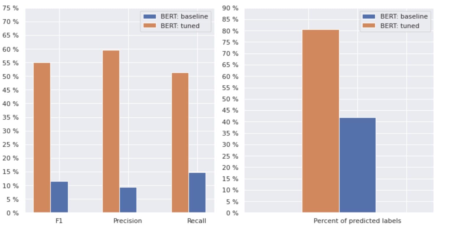
Figure 3. Comparison metrics by baseline and newer approach.
By comparing the metrics that are relevant for classification, we see a significant increase in performance measures almost by 5-6 times:
The F1 score increased from 12% → 55%, while Precision increased from 9% → 59% and Recall increased from 15% → 51%.
With the changes shown in the right graph in Figure 3, we can now predict 80% of the classes.
Slices of classes
We divided our labels into four groups: HEAD, MEDIUM, TAIL, and ZERO. Each group contains labels with a similar amount of supporting data observations.
As seen in Figure 4, the distributions of the groups are distinct. The rose box (HEAD) has a negatively skewed distribution, the middlebox (MEDIUM) has a positively skewed distribution, and the green box (TAIL) appears to have a normal distribution.
All groups also have outliers, which are points outside the whiskers in the box plot. The HEAD group has a major impact on a MAJOR class.
Additionally, we have identified a separate group named "ZERO" which contains labels that the model was unable to learn and cannot recognize due to the minimal number of occurrences in the dataset (less than 3% of all observations).
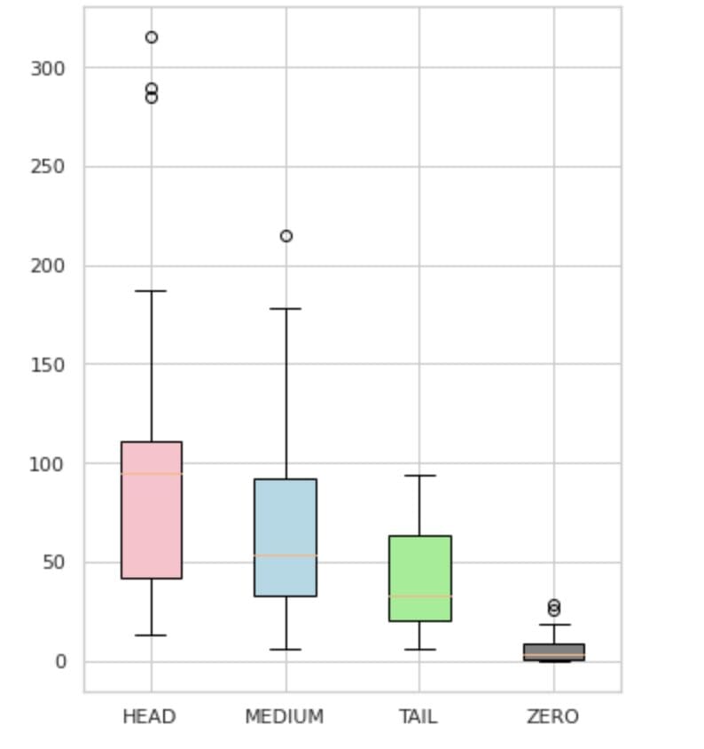
Figure 4. Label counts vs. groups
Table 2 provides information about metrics per each group of labels for the test subset of data.

Table 2. Metrics per group.
- The HEAD group contains 21 labels with an average of 112 support observations per label. This group is impacted by outliers and, due to its high representation in the dataset, its metrics are high: F1 - 73%, Precision - 71%, Recall - 75%.
- The MEDIUM group consists of 44 labels with an average support of 67 observations, which is approximately two times lower than the HEAD group. The metrics for this group are expected to decrease by 50%: F1 - 52%, Precision - 56%, Recall - 51%.
- The TAIL group has the largest number of classes, but all are poorly represented in the dataset, with an average of 40 support observations per label. As a result, the metrics drop significantly: F1 - 21%, Precision - 32%, Recall - 16%.
- The ZERO group includes classes that the model cannot recognize at all, potentially due to their low occurrence in the dataset. Each of the 24 labels in this group has an average of 7 support observations.
Figure 5 visualizes the information presented in Table 2, providing a visual representation of the metrics per group of labels.
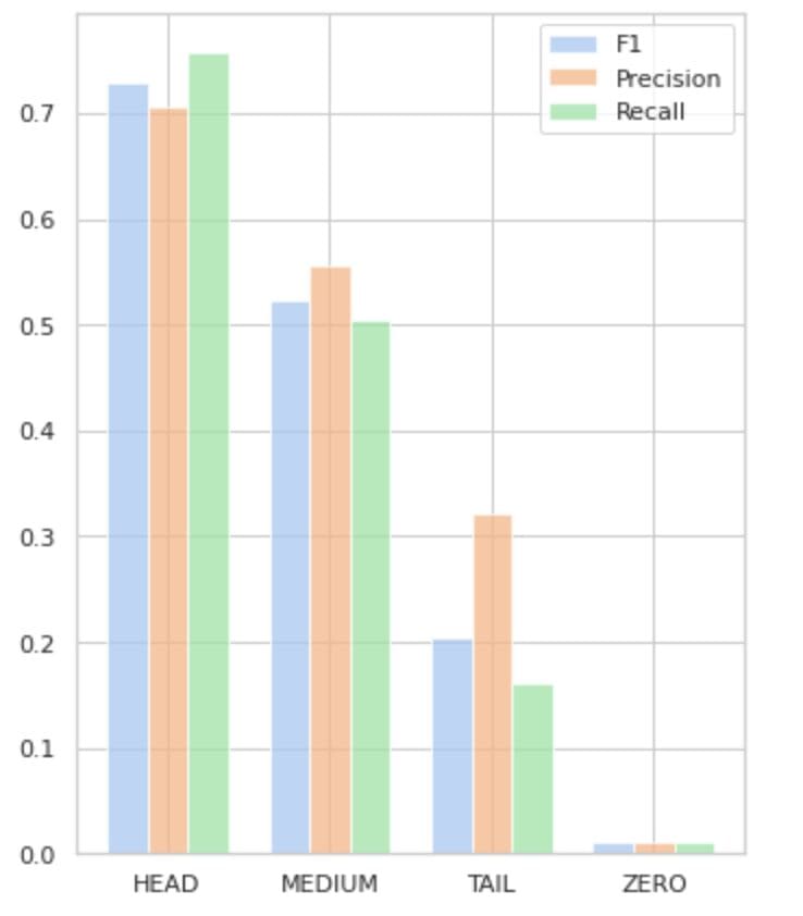
Figure 5. Metrics vs. label groups. All ZERO values = 0.
Conclusion
In this comprehensive article, we have demonstrated that a seemingly simple task of multi-label text classification can be challenging when traditional methods are applied. We have proposed the use of distribution-balancing loss functions to tackle the issue of class imbalance.
We have compared the performance of our proposed approach to the classic method, and evaluated it using real-world business metrics. The results demonstrate that utilizing loss functions to address class imbalances and label co-occurrences offer a viable solution for multi-label text classification.
The proposed use case highlights the importance of considering different approaches and techniques when dealing with multi-label text classification, and the potential benefits of distribution-balancing loss functions in addressing class imbalances.
If you are facing a similar issue and seeking to streamline document processing operations within your organization, please contact me or the Provectus team. We will be happy to assist you in finding more efficient methods for automating your processes.
Oleksii Babych is a Machine Learning Engineer at Provectus. With a background in physics, he possesses excellent analytical and math skills, and has gained valuable experience through scientific research and international conference presentations, including SPIE Photonics West. Oleksii specializes in creating end-to-end, large-scale AI/ML solutions for healthcare and fintech industries. He is involved in every stage of the ML development life cycle, from identifying business problems to deploying and running production ML models.
Rinat Akhmetov is the ML Solution Architect at Provectus. With a solid practical background in Machine Learning (especially in Computer Vision), Rinat is a nerd, data enthusiast, software engineer, and workaholic whose second biggest passion is programming. At Provectus, Rinat is in charge of the discovery and proof of concept phases, and leads the execution of complex AI projects.