Image from Bing Image Creator
Introduction
Who hasn’t been amused by technological advancements particularly in artificial intelligence, from Alexa to Tesla self-driving cars and a myriad other innovations? I marvel at the advancements every other day but what’s even more interesting is, when you get to have an idea of what underpins those innovations. Welcome to Artificial Intelligence and to the endless possibilities of deep learning. If you’ve been wondering what it is, then you’re home.
In this tutorial, I’ll deconstruct the terminology and take you through how to perform a deep learning task in R. To note, this article will assume that you have some basic understanding of machine learning concepts such as regression, classification, and clustering.
Let’s start with definitions of some terminologies surrounding the concept of deep learning:
Deep learning is a branch of machine learning that teaches computers to mimic the cognitive functions of the human brain. This is achieved through the use of artificial neural networks that help to unpack complex patterns in data sets. With deep learning, a computer can classify sounds, images, or even texts.
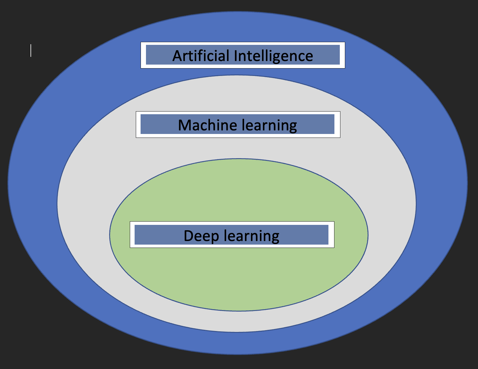
Before we dive into the specifics of Deep learning, it would be nice to understand what machine learning and artificial intelligence are and how the three concepts relate to each other.
Artificial intelligence: This is a branch of computer science that is concerned with the development of machines whose functioning mimics the human brain.
Machine learning: This is a subset of Artificial Intelligence that enables computers to learn from data.
With the above definitions, we now have an idea of how deep learning relates to artificial intelligence and machine learning.
The diagram below will help show the relationship.
Two crucial things to note about deep learning are:
- Requires huge volumes of data
- Requires high-performance computing power
Neural Networks
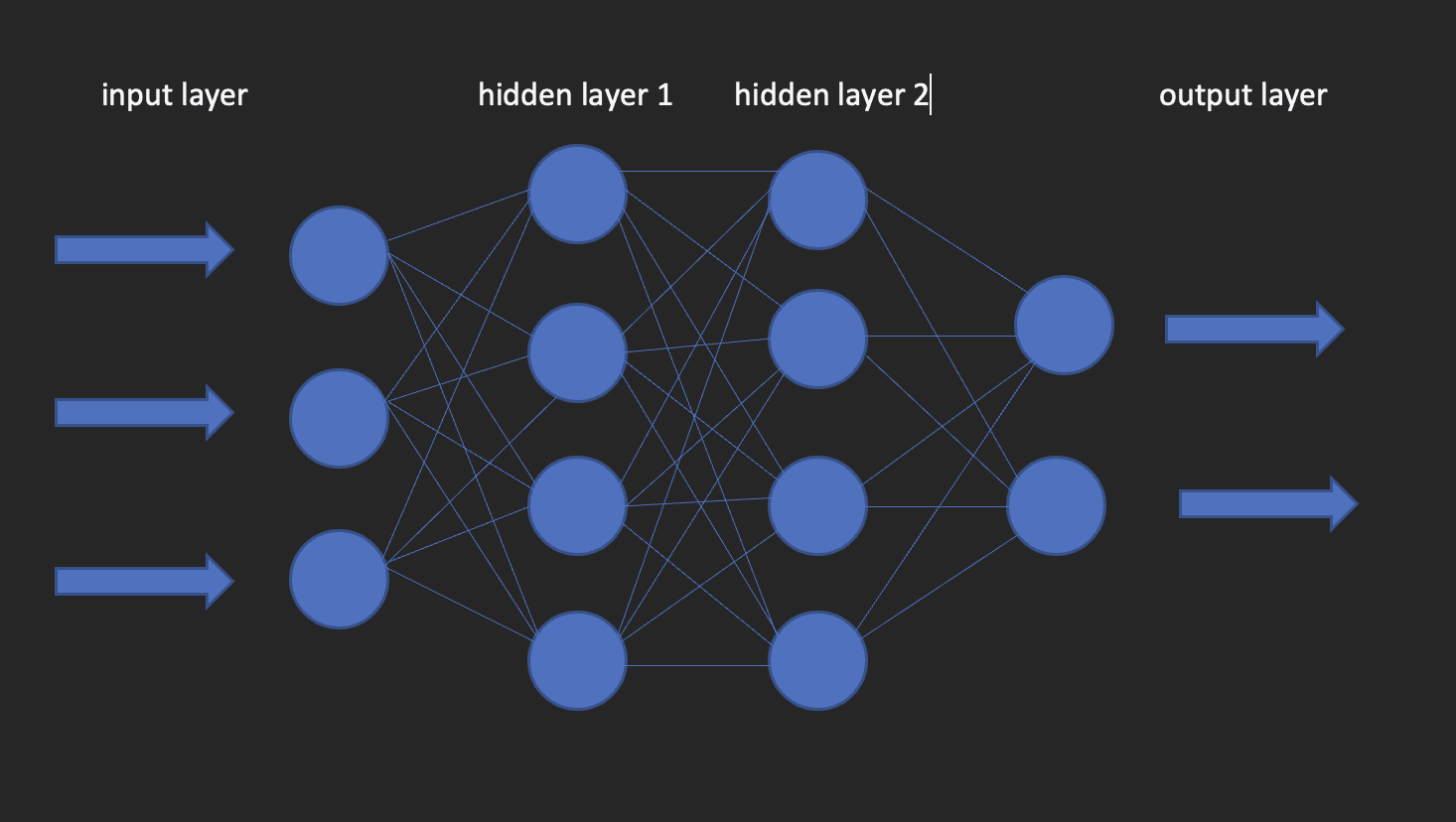
These are the building blocks of deep learning models. As the name suggests, the word neural comes from neurons, just like the neurons of the human brain. Actually, the architecture of deep neural networks gets its inspiration from the structure of the human brain.
A neural network has an input layer, one hidden layer and an output layer. This network is called a shallow neural network. When we have more than one hidden layer, it becomes a deep neural network, where the layers could be as many as 100’s.
The image below shows what a neural network looks like.
This brings us to the question of how to build deep learning models in R? Enter kera!
Keras is an open-source deep learning library that makes it easy to use neural networks in machine learning. This library is a wrapper that uses TensorFlow as a backend engine. However, there are other options for the backend such as Theano or CNTK.
Let us now install both TensorFlow and Keras.
Start with creating a virtual environment using reticulate
library(reticulate)
virtualenv_create("virtualenv", python = "/path/to/your/python3")

install.packages(“tensorflow”) #This is only done once!

library(tensorflow)

install_tensorflow(envname = "/path/to/your/virtualenv", version = "cpu")

install.packages(“keras”) #do this once!

library(keras)

install_keras(envname = "/path/to/your/virtualenv")

# confirm the installation was successful
tf$constant("Hello TensorFlow!")
Now that our configurations are set, we can head over to how we can use deep learning to solve a classification problem.
Brief about the Data
The data I’ll use for this tutorial is from an ongoing Salary Survey done by https://www.askamanager.org.
The main question asked in the form is how much money do you make, plus a couple of more details such as industry, age, years of experience, etc. The details are collected into a Google sheet from which I obtained the data.
The problem we want to solve with data is to be able to come up with a deep learning model that predicts how much someone could potentially earn given information such as age, gender, years of experience, and highest level of education.
Load the libraries that we’ll require.
library(dplyr)
library(keras)
library(caTools)
Import the data
url <- “https://raw.githubusercontent.com/oyogo/salary_dashboard/master/data/salary_data_cleaned.csv”

salary_data <- read.csv(url)
Select the columns that we need
salary_data <- salary_data %>% select(age,professional_experience_years,gender,highest_edu_level,annual_salary)
Data Cleaning
Remember the computer science GIGO concept? (Garbage in Garbage Out). Well, this concept is perfectly applicable here as it is in other domains. The results of our training will largely depend on the quality of the data we use. This is what brings data cleaning and transformation, a critical step in any Data Science project.
Some of the key issues data cleaning seeks to address are; consistency, missing values, spelling issues, outliers, and data types. I won’t go into the details on how those issues are tackled and this is for the simple reason of not wanting to digress from the subject matter of this article. Therefore, I’ll use the cleaned version of the data but if you’re interested in knowing how the cleaning bit was handled, check this article out.
Data Transformations
Artificial neural networks accept numeric variables only and seeing that some of our variables are of categorical nature, we will need to encode such into numbers. This is what forms part of the data preprocessing step, which is necessary because more often than not, you won’t get data that is ready for modeling.
# create an encoder function
encode_ordinal <- function(x, order = unique(x)) {
  x <- as.numeric(factor(x, levels = order, exclude = NULL))
}

salary_data <- salary_data %>% mutate(
  highest_edu_level = encode_ordinal(highest_edu_level, order = c("High School","College degree","Master's degree","Professional degree (MD, JD, etc.)","PhD")),
  professional_experience_years = encode_ordinal(professional_experience_years,
  order = c("1 year or less", "2 - 4 years","5-7 years",  "8 - 10 years", "11 - 20 years", "21 - 30 years", "31 - 40 years", "41 years or more")),
  age = encode_ordinal(age, order = c( "under 18", "18-24","25-34", "35-44", "45-54", "55-64","65 or over")),
  gender = case_when(gender== "Woman" ~ 0,
                 	gender == "Man" ~ 1))
Seeing that we want to solve a classification, we need to categorize the annual salary into two classes so that we use it as the response variable.
salary_data <- salary_data %>%
  mutate(categories = case_when(
	annual_salary <= 100000 ~ 0,
	annual_salary > 100000 ~ 1))

salary_data <- salary_data %>% select(-annual_salary)
Split the Data
As in the basic machine learning approaches; regression, classification, and clustering, we will need to split our data into training and testing sets. We do this using the 80-20 rules, which is 80% of the dataset for training and 20% for testing. This is not cast on stones, as you can decide to use any split ratios as you see fit, but keep in mind that the training set should have a good share of the percentages.
set.seed(123)

sample_split <- sample.split(Y = salary_data$categories, SplitRatio = 0.7)
train_set <- subset(x=salary_data, sample_split == TRUE)
test_set <- subset(x = salary_data, sample_split == FALSE)

y_train <- train_set$categories
y_test <- test_set$categories
x_train <- train_set %>% select(-categories)
x_test <- test_set %>% select(-categories)
Keras takes in inputs in the form of matrices or arrays. We use the as.matrix function for the conversion. Also, we need to scale the predictor variables and then we convert the response variable to categorical data type.
x <- as.matrix(apply(x_train, 2, function(x) (x-min(x))/(max(x) - min(x))))

y <- to_categorical(y_train, num_classes = 2)
Instantiate the model
Create a sequential model onto which we’ll add layers using the pipe operator.
model = keras_model_sequential()
Configure the Layers
The input_shape specifies the shape of the input data. In our case, we have obtained that using the ncol function. activation: Here we specify the activation function; a mathematical function that transforms the output to a desired non-linear format before passing it to the next layer.
units: the number of neurons in each layer of the neural network.
model %>%
  layer_dense(input_shape = ncol(x), units = 10, activation = "relu") %>%
  layer_dense(units = 10, activation = "relu") %>%
  layer_dense(units = 2, activation = "sigmoid")
Configure the Model Learning Process
We use the compile method to do this. The function takes three arguments;
optimizer : This object specifies the training procedure. loss : This is the function to minimize during optimization. Options available are mse (mean square error), binary_crossentropy and categorical_crossentropy.
metrics : What we use to monitor the training. Accuracy for classification problems.
model %>%
  compile(
	loss = "binary_crossentropy",
	optimizer = "adagrad",
	metrics = "accuracy"
)
Model Fitting
We can now fit the model using the fit method from Keras. Some of the arguments that fit takes in are:
epochs : An epoch is an iteration over the training dataset.
batch_size : The model slices the matrix/array passed to it into smaller batches over which it iterates during training.
validation_split : Keras will need to slice a portion of the training data to obtain a validation set that will be used to evaluate model performance for each epoch.
shuffle : Here you Indicate whether you want to shuffle your training data before each epoch.
fit = model %>%
  fit(
	x = x,
	y = y,
	shuffle = T,
	validation_split = 0.2,
	epochs = 100,
	batch_size = 5
)
Evaluate the model
To obtain the accuracy value of the model use the evaluate function as below.
y_test <- to_categorical(y_test, num_classes = 2)
model %>% evaluate(as.matrix(x_test),y_test)
Prediction
To predict on new data use the predict_classes function from keras library as below.
model %>% predict(as.matrix(x_test))
Conclusion
This article has taken you through the basics of deep learning with Keras in R. You’re welcome to dive deeper for better understanding, play around with the parameters, get your hands dirty with data preparation, and perhaps scale the computations by leveraging the power of cloud computing.
Clinton Oyogo writer at Saturn Cloud believes that analyzing data for actionable insights is a crucial part of his day-to-day work. With his skills in data visualization, data wrangling, and machine learning, he takes pride in his work as a data scientist.
Original. Reposted with permission.