Applying Descriptive and Inferential Statistics in Python
As you progress in your data science journey, here are the elementary statistics you should know.

Photo by Mikael Blomkvist
Statistics is a field encompassing activities from collecting data and data analysis to data interpretation. It’s a study field to help the concerned party decide when facing uncertainty.
Two major branches in the statistics field are descriptive and Inferential. Descriptive statistics is a branch related to data summarization using various manners, such as summary statistics, visualization, and tables. While inferential statistics are more about population generalization based on the data sample.
This article will walk through a few important concepts in Descriptive and Inferential statistics with a Python example. Let’s get into it.
Descriptive Statistics
As I have mentioned before, descriptive statistics focus on data summarization. It’s the science of processing raw data into meaningful information. Descriptive statistics can be performed with graphs, tables, or summary statistics. However, summary statistics is the most popular way to do descriptive statistics, so we would focus on this.
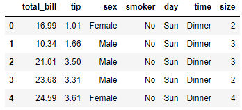
For our example, we would use the following dataset example.
import pandas as pd
import numpy as np
import seaborn as sns

tips = sns.load_dataset('tips')
tips.head()
With this data, we would explore descriptive statistics. In the summary statistics, there are two most used: Measures of Central Tendency and Measures of Spread.
Measures of Central Tendency
Central tendency is the center of the data distribution or the dataset. The measures of central tendency are the activity to acquire or describe the center distribution of our data. The measures of central tendency would give a singular value that defines the data's central position.
Within measures of Central Tendency, there are three popular measurements:
1. Mean
Mean or average is a method to produce a singular value output representing our data's most common value. However, the mean is not necessarily the value observed in our data.
We can calculate the mean by taking a sum of the existing values in our data and dividing it by the number of values. We can represent the mean with the following equation:
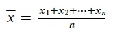
Image by Author
In Python, we can calculate data mean with the following code.
round(tips['tip'].mean(), 3)
2.998
Using the pandas series attribute, we can obtain the data mean. We also round the data to make the data reading easier.
Mean has a disadvantage as a measure of central tendency because it is affected heavily by the outlier, which could skew the summary statistic and not best represent the actual situation. In skewed cases, we can use the median.
2. Median
The median is the singular value positioned in the middle of the data if we sort them, representing the data's halfway point position (50%). As a measurement of central tendency, the median is preferable when the data is skewed because it could represent the data center, as the outlier or skewed values do not strongly influence it.
The median is calculated by arranging all the data values in ascending order and finding the middle value. The median is the middle value for an odd number of data values, but the median is the average of the two middle values for an even number of data values.
We can calculate the Median with Python using the following code.
tips['tip'].median()
2.9
3. Mode
Mode is the highest frequency or most occurring value within the data. The data can have a single mode (unimodal), multiple modes (multimodal), or no mode at all (if there are no repeating values).
Mode is usually used for categorical data but can be used in numerical data. For categorical data, though, it might only use the mode. This is because categorical data do not have any numerical values to calculate the mean and median.
We can calculate the data Mode with the following code.
tips['day'].mode()
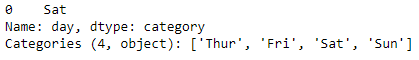
The result is the series object with categorical type values. The ‘Sat’ value is the only one that comes out because it’s the data mode.
Measures of Spread
The measures of spread (or variability, dispersion) is a measurement to describe data value spreads. The measurement provides information on how our data values vary within the dataset. It is often used with the measures of central tendency as they complement the overall data information.
The measures of the spread also help understand how well our measures of central tendency output. For example, a higher data spread might indicate a significant deviation between the observed data, and the data mean might not best represent the data.
Here are various measures of spread to use.
- Range
The range is the difference between the data's largest (Max) and smallest value (Min). It’s the most direct measurement because the information only uses two aspects of the data.
The usage might be limited because it doesn’t tell much about the data distribution, but it might help our assumption if we have a certain threshold to use for our data. Let’s try to calculate the data range with Python.
tips['tip'].max() - tips['tip'].min()
9.0
2. Variance
Variance is a measurement of spread that informs our data spreads based on the data mean. We calculate variance by squaring the differences of each value to the data mean and dividing it by the number of the data values. As we usually work with data samples and not populations, we subtract the number of the data values by one. The equation for sample variance is in the image below.
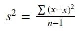
Image by Author
Variance can be interpreted as a value indicating how far the data is spread to the mean and each other. Higher variance means a wider data spread. However, variance calculation is sensitive to the outlier because we squared the scores' deviations from the mean; it means we gave more weight to the outlier.
Let’s try to calculate data variance with Python.
round(tips['tip'].var(),3)
1.914
The variance above might suggest a high variance in our data, but we might want to use the Standard Deviation to have an actual value for our data spread measurement.
3. Standard Deviation
Standard deviation is the most common way to measure the data spread, and it’s calculated by taking the variance's square root.
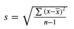
Image by Author
The difference between variance and the standard deviation is in the information their value gave. Variance value only indicates how spread our values were from the mean, and the variance unit differs from the original value as we squared the original values. However, the standard deviation value is the same unit as the original data value, which means the standard deviation value can be used directly to measure our data's spread.
Let’s try to calculate the Standard Deviation with the following code.
round(tips['tip'].std(),3)
1.384
One of the most common applications of standard deviation is to estimate the data interval. We can estimate the data interval using the empirical rule or the 68–95–99.7 rule. The empirical rule stated that 68% of data is estimated to fall within the data mean ± one STD, 95% of data is mean ± two STD, and 99.7% of data is within mean ± three STD. Outside of this interval, it could be assumed as an outlier.
4. Interquartile Range
Interquartile Range (IQR) is a measure of spread calculated using the differences between the first and third quartile data. The quartile itself is a value that divides the data into four different parts. To understand better, let’s take a look at the following image.
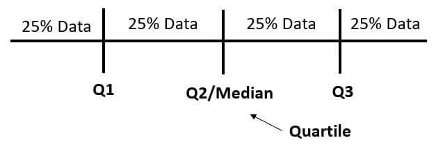
Image by Author
The quartile is the value that divides the data rather than the result of the division. We can use the following code to find the quartile values and IQR.
q1, q3= np.percentile(tips['tip'], [25 ,75])
iqr = q3 - q1

print(f'Q1: {q1}\nQ3: {q3}\nIQR: {iqr}')
Q1: 2.0

Q3: 3.5625

IQR: 1.5625
Using the numpy percentile function, we can acquire the quartile. By subtracting the third quartile and the first quartile, we get the IQR.
IQR can be used to identify the data outlier by taking the IQR value and calculating the data upper/lower limit. The upper limit formula is the Q3 + 1.5 * IQR, while the lower limit is the Q1 - 1.5 * IQR. Any values passing this limit would be considered outliers.
To understand better, we can use the boxplot to understand the IQR outlier detection.
sns.boxplot(tips['tip'])
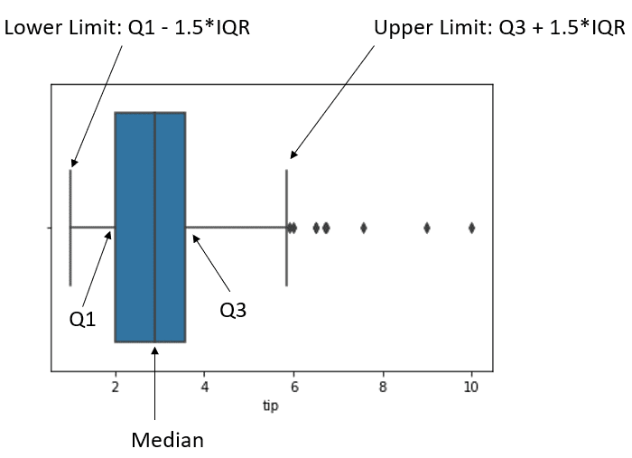
The image above shows the data boxplot and the data position. The black dot after the upper limit is what we consider an outlier.
Inferential Statistics
Inferential statistics is a branch that generalizes the population information based on the data sample it comes from. Inferential statistics is used because it is often impossible to get the whole data population, and we need to make inferential from the data sample. For example, we want to understand how Indonesia people’s opinions about AI. However, the study would take too long if we surveyed everyone in the Indonesian population. Hence, we use the sample data representing the population and make inferences about the Indonesian population's opinion about AI.
Let’s explore various Inferential Statistics we could use.
1. Standard Error
The standard error is an inferential statistics measurement to estimate the true population parameter given the sample statistic. The standard error information is how the sample statistic would vary if we repeat the experiment with the data samples from the same population.
The standard error of the mean (SEM) is the most commonly used type of standard error as it tells how well the mean would represent the population given the sample data. To calculate SEM, we would use the following equation.
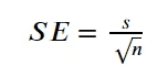
Image by Author
Standard error of Mean would use standard deviation for the calculation. The standard error of the data would be smaller the higher the number of the sample, where smaller SE means that our sample would be great to represent the data population.
To get the standard error of the mean, we can use the following code.
from scipy.stats import sem

round(sem(tips['tip']),3)
0.089
We often report SEM with the data mean where the true mean population would estimated to fall within the mean±SEM.
data_mean = round(tips['tip'].mean(),3)
data_sem = round(sem(tips['tip']),3)
print(f'The true population mean is estimated to fall within the range of {data_mean+data_sem} to {data_mean-data_sem}')
The true population mean is estimated to fall within the range of 3.087 to 2.9090000000000003
2. Confidence interval
Confidence interval is also used to estimate the true population parameter, but it introduces the confidence level. The confidence level estimates the true population parameters range with a certain confidence percentage.
In statistics, confidence can be described as a probability. For example, a confidence interval with a 90% confidence level means that the true mean population estimate would be within the confidence interval's upper and lower values 90 out of 100 times. CI is calculated with the following formula.
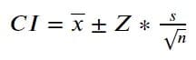
Image by Author
The formula above has a familiar notation except Z. The Z notation is a z-score acquired by defining the confidence level (e.g., 95%) and using the z-critical value table to determine the z-score (1.96 for a confidence level of 95%). Additionally, if our sample is small or below 30, we are supposed to use the t-distribution table.
We can use the following code to get the CI with Python.
import scipy.stats as st

st.norm.interval(confidence=0.95, loc=data_mean, scale=data_sem)
(2.8246682963727068, 3.171889080676473)
The above result could be interpreted that our data true population mean falls between the range 2.82 to 3.17 with 95% confidence level.
3. Hypothesis Testing
Hypothesis testing is a method in inferential statistics to conclude from data samples about the population. The estimated population could be the population parameter or the probability.
In Hypothesis testing, we need to have an assumption called the null hypothesis (H0), and the alternative hypothesis (Ha). Null hypothesis and alternative hypothesis are always opposite of each other. The hypothesis testing procedure then would use the sample data to determine whether or not the null hypothesis can be rejected or we fail to reject it (which means we accept the alternative hypothesis).
When we perform a hypothesis testing method to see if the null hypothesis must be rejected, we need to determine the significance level. The level of significance is the type 1 error ( rejecting H0 when H0 is true) maximum probability that is allowed to happen in the test. Usually, the significance level is 0.05 or 0.01.
To draw a conclusion from the sample, hypothesis testing uses the P-value when assuming the null hypothesis is true to measure how likely the sample results are. When the P-value is smaller than the significance level, we reject the null hypothesis; otherwise, we can’t reject it.
Hypothesis testing is a method that can be performed in any population parameter and could be performed on multiple parameters as well. For example, the below code would perform a t-test on two different populations to see if this data is significantly different than the other.
st.ttest_ind(tips[tips['sex'] == 'Male']['tip'], tips[tips['sex'] == 'Female']['tip'])
Ttest_indResult(statistic=1.387859705421269, pvalue=0.16645623503456755)
In the t-test, we compare the means between two groups (pairwise test). The null hypothesis for the t-test is that there are no differences between the two groups' mean, while the alternative hypothesis is that there are differences between the two groups' mean.
The t-test result shows that the tip between the Male and Female is not significantly different because the P-value is above 0.05 significance level. It means we failed to reject the null hypothesis and conclude that there are no differences between the two groups' means.
Of course, the test above only simplifies the hypothesis testing example. There are many assumptions we need to know when we perform hypothesis testing, and there are many tests that we can do to fulfill our needs.
Conclusion
There are two major branches of statistics field which we need to know: descriptive and Inferential statistics. Descriptive statistics is concerned with summarizing data, while inferential statistics tackle data generalization to make inferences about the population. In this article, we have discussed descriptive and inferential statistics while having examples with the Python code.
Cornellius Yudha Wijaya is a data science assistant manager and data writer. While working full-time at Allianz Indonesia, he loves to share Python and Data tips via social media and writing media.