9 Key Deep Learning Papers, Explained

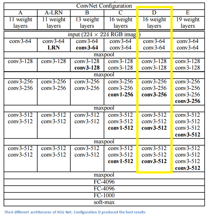
3. VGG Net (2014)

 
Simplicity and depth. That’s what a model created in 2014 (weren’t the winners of ILSVRC 2014) best utilized with its 7.3% error rate. Karen Simonyan and Andrew Zisserman of the University of Oxford created a 19 layer CNN that strictly used 3x3 filters with stride and pad of 1, along with 2x2 maxpooling layers with stride 2. Simple enough right?

Main Points

• The use of only 3x3 sized filters is quite different from AlexNet’s 11x11 filters in the first layer and ZF Net’s 7x7 filters. The authors’ reasoning is that the combination of two 3x3 conv layers has an effective receptive field of 5x5. This in turn simulates a larger filter while keeping the benefits of smaller filter sizes. One of the benefits is a decrease in the number of parameters. Also, with two conv layers, we’re able to use two ReLU layers instead of one.
• 3 conv layers back to back have an effective receptive field of 7x7.
• As the spatial size of the input volumes at each layer decrease (result of the conv and pool layers), the depth of the volumes increase due to the increased number of filters as you go down the network.
• Interesting to notice that the number of filters doubles after each maxpool layer. This reinforces the idea of shrinking spatial dimensions, but growing depth.
• Worked well on both image classification and localization tasks. The authors used a form of localization as regression (see page 10 of the paper for all details).
• Built model with the Caffe toolbox.
• Used scale jittering as one data augmentation technique during training.
• Used ReLU layers after each conv layer and trained with batch gradient descent.
• Trained on 4 Nvidia Titan Black GPUs for two to three weeks.

Why It’s Important

VGG Net is one of the most influential papers in my mind because it reinforced the notion that convolutional neural networks have to have a deep network of layers in order for this hierarchical representation of visual data to work. Keep it deep. Keep it simple.

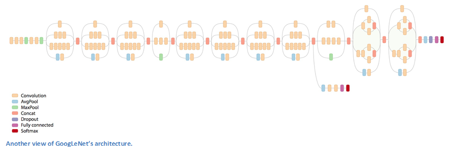
4. GoogLeNet (2015)

 
You know that idea of simplicity in network architecture that we just talked about? Well, Google kind of threw that out the window with the introduction of the Inception module. GoogLeNet is a 22 layer CNN and was the winner of ILSVRC 2014 with a top 5 error rate of 6.7%. To my knowledge, this was one of the first CNN architectures that really strayed from the general approach of simply stacking conv and pooling layers on top of each other in a sequential structure. The authors of the paper also emphasized that this new model places notable consideration on memory and power usage (Important note that I sometimes forget too: Stacking all of these layers and adding huge numbers of filters has a computational and memory cost, as well as an increased chance of overfitting).

Inception Module

When we first take a look at the structure of GoogLeNet, we notice immediately that not everything is happening sequentially, as seen in previous architectures. We have pieces of the network that are happening in parallel.

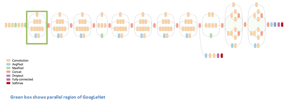
This box is called an Inception module. Let’s take a closer look at what it’s made of.

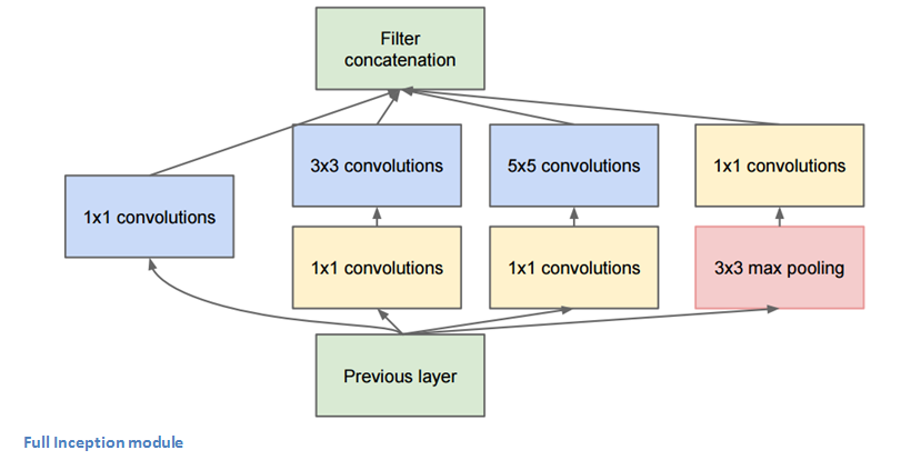
The bottom green box is our input and the top one is the output of the model (Turning this picture right 90 degrees would let you visualize the model in relation to the last picture which shows the full network). Basically, at each layer of a traditional ConvNet, you have to make a choice of whether to have a pooling operation or a conv operation (there is also the choice of filter size). What an Inception module allows you to do is perform all of these operations in parallel. In fact, this was exactly the “naïve” idea that the authors came up with.

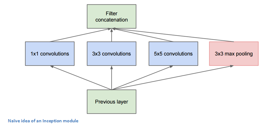
Now, why doesn’t this work? It would lead to way too many outputs. We would end up with an extremely large depth channel for the output volume. The way that the authors address this is by adding 1x1 conv operations before the 3x3 and 5x5 layers. The 1x1 convolutions (or network in network layer) provide a method of dimensionality reduction. For example, let’s say you had an input volume of 100x100x60 (This isn’t necessarily the dimensions of the image, just the input to any layer of the network). Applying 20 filters of 1x1 convolution would allow you to reduce the volume to 100x100x20. This means that the 3x3 and 5x5 convolutions won’t have as large of a volume to deal with. This can be thought of as a “pooling of features” because we are reducing the depth of the volume, similar to how we reduce the dimensions of height and width with normal maxpooling layers.  Another note is that these 1x1 conv layers are followed by ReLU units which definitely can’t hurt (See Aaditya Prakash’s great post for more info on the effectiveness of 1x1 convolutions). Check out this video for a great visualization of the filter concatenation at the end.

You may be asking yourself “How does this architecture help?”. Well, you have a module that consists of a network in network layer, a medium sized filter convolution, a large sized filter convolution, and a pooling operation. The network in network conv is able to extract information about the very fine grain details in the volume, while the 5x5 filter is able to cover a large receptive field of the input, and thus able to extract its information as well. You also have a pooling operation that helps to reduce spatial sizes and combat overfitting. On top of all of that, you have ReLUs after each conv layer, which help improve the nonlinearity of the network. Basically, the network is able to perform the functions of these different operations while still remaining computationally considerate. The paper does also give more of a high level reasoning that involves topics like sparsity and dense connections (read Sections 3 and 4 of the paper. Still not totally clear to me, but if anybody has any insights, I’d love to hear them in the comments!).

Main Points

• Used 9 Inception modules in the whole architecture, with over 100 layers in total! Now that is deep…
• No use of fully connected layers! They use an average pool instead, to go from a 7x7x1024 volume to a 1x1x1024 volume. This saves a huge number of parameters.
• Uses 12x fewer parameters than AlexNet.
• During testing, multiple crops of the same image were created, fed into the network, and the softmax probabilities were averaged to give us the final solution.
• Utilized concepts from R-CNN (a paper we’ll discuss later) for their detection model.
• There are updated versions to the Inception module (Versions 6 and 7).
• Trained on “a few high-end GPUs within a week”.

Why It’s Important

GoogLeNet was one of the first models that introduced the idea that CNN layers didn’t always have to be stacked up sequentially. Coming up with the Inception module, the authors showed that a creative structuring of layers can lead to improved performance and computationally efficiency. This paper has really set the stage for some amazing architectures that we could see in the coming years.

5. Microsoft ResNet (2015)

 
Imagine a deep CNN architecture. Take that, double the number of layers, add a couple more, and it still probably isn’t as deep as the ResNet architecture that Microsoft Research Asia came up with in late 2015. ResNet is a new 152 layer network architecture that set new records in classification, detection, and localization through one incredible architecture. Aside from the new record in terms of number of layers, ResNet won ILSVRC 2015 with an incredible error rate of 3.6% (Depending on their skill and expertise, humans generally hover around a 5-10% error rate. See Andrej Karpathy’s great post on his experiences with competing against ConvNets on the ImageNet challenge).

Residual Block

The idea behind a residual block is that you have your input x go through conv-relu-conv series. This will give you some F(x). That result is then added to the original input x. Let’s call that H(x) = F(x) + x. In traditional CNNs, your H(x) would just be equal to F(x) right? So, instead of just computing that transformation (straight from x to F(x)), we’re computing the term that you have to add, F(x), to your input, x. Basically, the mini module shown below is computing a “delta” or a slight change to the original input x to get a slightly altered representation (When we think of traditional CNNs, we go from x to F(x) which is a completely new representation that doesn’t keep any information about the original x). The authors believe that “it is easier to optimize the residual mapping than to optimize the original, unreferenced mapping”.

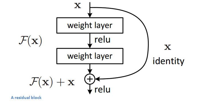
Another reason for why this residual block might be effective is that during the backward pass of backpropagation, the gradient will flow easily through the effective because we have addition operations, which distributes the gradient.

Main Points

• “Ultra-deep” – Yann LeCun.
• 152 layers…
• Interesting note that after only the first 2 layers, the spatial size gets compressed from an input volume of 224x224 to a 56x56 volume.
• Authors claim that a naïve increase of layers in plain nets result in higher training and test error (Figure 1 in the paper).
• The group tried a 1202-layer network, but got a lower test accuracy, presumably due to overfitting.
• Trained on an 8 GPU machine for two to three weeks.

Why It’s Important

3.6% error rate. That itself should be enough to convince you. The ResNet model is the best CNN architecture that we currently have and is a great innovation for the idea of residual learning. With error rates dropping every year since 2012, I’m skeptical about whether or not they will go down for ILSVRC 2016. I believe we’ve gotten to the point where stacking more layers on top of each other isn’t going to result in a substantial performance boost. There would definitely have to be creative new architectures like we’ve seen the last 2 years. On September 16th, the results for this year’s competition will be released. Mark your calendar.

Bonus: ResNets inside of ResNets. Yeah. I went there.