Understanding Basic Concepts and Dispersion

By Saurabh Agrawal and Prasad Pande (RideOnData).

In a previous post Statistics – Understanding the Levels of Measurement, we have seen what variables are, and how do we measure them based on the different levels of measurement. In this post, we will talk about some of the basic concepts that are important to get started with statistics and then dive deep into the concept of dispersion.

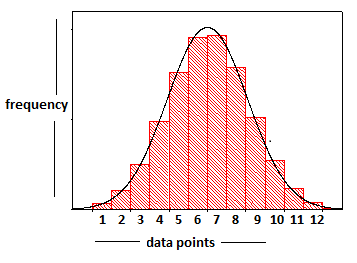
Histogram:

A histogram is a graphical representation of the distribution of numerical data. We know the basic bar graph, but in a histogram, all the bars involved are connected or they touch each other – meaning that there is no gap between the points. Eg: Consider we have some data points (i.e values of the variable that we measured), we create this histogram by plotting the data points against their corresponding frequency of occurrence in our random sample. We then draw the distribution curve by connecting the midpoints of the bars in the histogram. So the important point to remember here is that there are bars sitting below that curve, and the process of drawing the distribution curve is: numbers to bars to curve.

Independent and Dependent Variables:

We have seen that a variable is nothing but a concept that can be measured, and its value may vary across the sample from case to case. The dependent and independent variables are used to represent the concept of cause and effect. Eg: consider two variables, say, calories_you_eat and your_weight. Now, your_weight depends on the calories_you_eat. So calories_you_eat in the independent variable and represents the cause, whereas your_weight is the dependent variable and represents the effect.

Central Tendency:

Central tendency represents the most typical value in a set of numbers. It is a way to summarize the data. So once we have our data, we want to describe it i.e use a number to describe the rest of the data. So our goal is to find the number that represents the rest of data or the point around which the data is clustered or distributed. Once we know this number, we can use it to compare the different groups of data. The technique used to measure the central tendency depends on the level of measurement of the variable. There are mainly three measures of central tendency – Mean, Median and Mode.

Mean is only appropriate with interval and ratio level data, and is the only measure of central tendency that incorporates all of the scores in the dataset. It is calculated by summing up the values of all the data points and then dividing by the number of data points.

Eg: 1,2,3,4,5 (mean = (1+2+3+4+5)/5 = 3)

Median is the data point that divides our data into upper and lower halves. So it is the value at the exact center of a distribution, so that 50% of cases are below and 50% are above the median. The median is appropriate for ordinal, interval, and ratio level variables, but not nominal variables. 

Eg: 1,2,3,4,5 (median = 3)

Mode is the category that has the maximum data points or the value that occurs most frequently. It is the only measure of central tendency that can be used with nominal variables, but can also be used with the ordinal, interval, and ratio variables. Eg: If we categorize the data points and observe that the category A has 20, B has 23 and C has 32 data points, then the mode is category C.

Dispersion:

Dispersion is used to measure the variability in the data or to see how spread out the data is. It measures how much the scores in a distribution vary from the typical score. So once we know the typical score of a set of values, we might want to know “how typical” it is of the entire group of data, or how much the scores vary from that typical score. This is measured by dispersion. When dispersion is low, the central tendency is more accurate or more representative of the data as majority of the data points are near the typical value, thus resulting in low dispersion and vice versa.

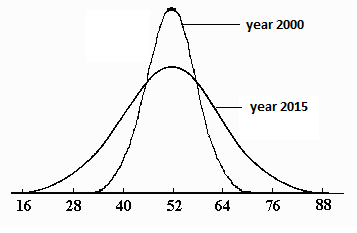
Measuring dispersion is important to validate the claims like – “The rich are getting richer, and poor are getting poorer”. Assume that we  measured the incomes of a random sample of population in the year 2000 and again in the year 2015. In this case, mean is not important to answer the question, because it can be the case that the two distributions have the same mean but different dispersion (i.e. spread) of data which is more important to answer this question.

Let the distribution of income in our  random samples from year 2000 and 2015 be represented by the two curves as shown in the diagram. We see that the two curves for the year 2015 and year 2000 have the same mean i.e. 52, but the curve for year 2015 is more spread out as compared to that for year 2000. Thus, as compared to 2000, there were more people in 2015 with higher and lower incomes which validates our claim.

Dispersion can be measured in a number of ways:

1. Range – The range of a dataset gives the difference between the largest and smallest value.  Therefore, the range only takes the two most extreme values into account and tells nothing about what falls in the middle.

   Range = (Max. Value – Min. Value)

2. Variation Ratio – When data is measured at the nominal level, we can only compare the size of each category represented in the dataset. Variation Ratio (VR) tells us how much variation there is in the dataset from the modal category. A low VR indicates that the data is concentrated more in the modal category and dispersion is less, whereas a high VR indicates that the data is more distributed across categories, thereby resulting into high dispersion.

   Variation Ratio = 1 – (#data points in modal category / #total data points in all categories)

3. Mean Deviation – The mean deviation gives us a measure of the typical difference (or deviation) from the mean.  If most data values are very similar to the mean, then the mean deviation score will be low, indicating high similarity within the data.  If there is great variation among scores, then the mean deviation score will be high, indicating low similarity within the data. Let Xi be the observed value of data point, X(bar) be the mean and N be the total data points.

   

4. Standard Deviation – The standard deviation of a dataset gives a measure of how each value in a dataset varies from the mean. This is very similar to the mean deviation, and indeed, gives us quite similar information, substantively. Let Xi be the observed value of data point, X(bar) be the mean and N be the total data points.

   

Thus, range tells us how far the extreme points of distribution are, and variation ratio tells us about the distribution of data in different categories relative to the modal category. Also, standard deviation and mean deviation tells us how data points in the distribution varies w.r.t the mean.

Original.

Related:

• Statistics – Understanding the Levels of Measurement
• 10 things statistics taught us about big data analysis
• Statistics Denial Myth: Repackaging Statistics With Straddling Terms