The Gentlest Introduction to Tensorflow – Part 2

By Soon Hin Khor, Co-organizer for Tokyo Tensorflow Meetup.

Editor's note: You may want to check out part 1 of this tutorial before proceeding.

Quick Review

 
In the previous article, we used Tensorflow (TF) to build and learn a linear regression model with a single feature so that given a feature value (house size/sqm), we can predict the outcome (house price/$).

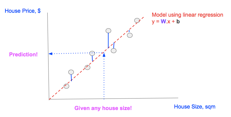
Here is the review with illustration below:

1. We have some data of house sizes & house prices (the gray round points)
2. We model the data using linear regression (the red dash line)
3. We find the ‘best’ model by training W, and b (of the linear regression model) to minimize the ‘cost’ (the sum of the length of vertical blue lines, which represent the differences between predictions and actual outcomes)
4. Given any house size, we can use the linear model to predict the house size (the dotted blue lines with arrows)

In machine learning (ML) literature, we come across the term ‘training’ very often, let us literally look at what that means in TF.

Linear Regression Modeling

Linear Model (in TF notation): y = tf.matmul(x,W) + b

The goal in linear regression is to find W, b, such that given any feature value (x), we can find the prediction (y) by substituting W, x, b values into the model.
However to find W, b that can give accurate predictions, we need to ‘train’ the model using available data (the multiple pairs of actual feature (x), and actual outcome (y_), note the underscore).

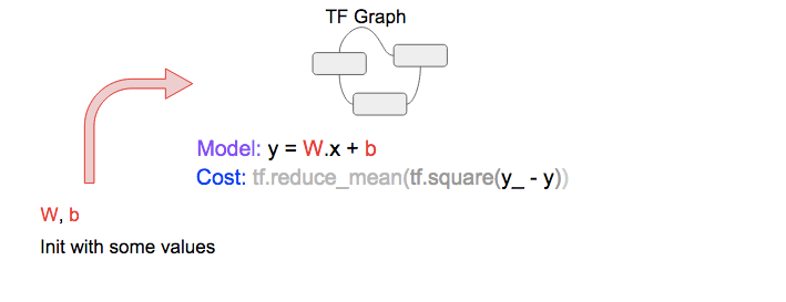
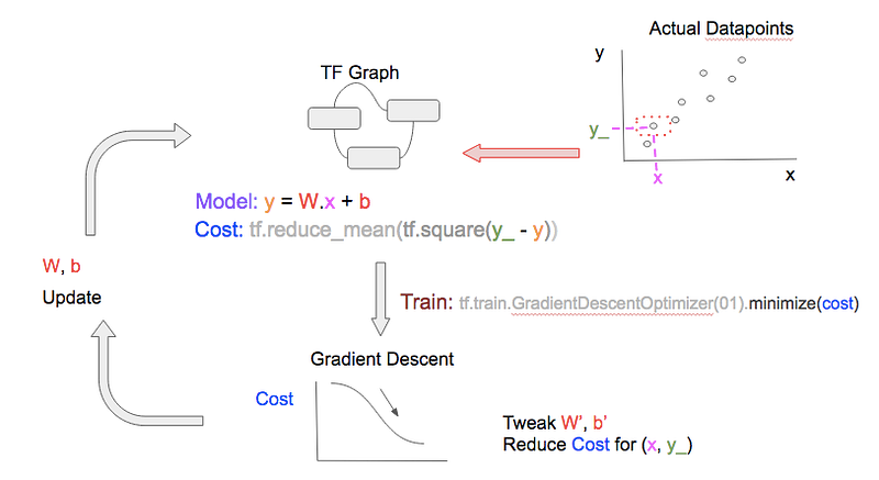
‘Training’ Illustrated

 
To find the best W, b values, we can initially start with any W, b values. We also need to define a cost function, which is a measure of the differencebetween the prediction (y) for given a feature value (x), and the actual outcome (y_) for that same feature value (x). For simplicity, we use leastminimum squared error (MSE) as our cost function.

Cost function (in TF notation): tf.reduce_mean(tf.square(y_ - y))

By minimizing the cost function, we can arrive at good W, b values.

Our code to do training is actually very simple and it is labelled with [A, B, C, D], which we will refer to later on. The full source is on Github.

# ... (snip) Variable/Constants declarations (snip) ...

# [A] TF.Graph
y = tf.matmul(x,W) + b
cost = tf.reduce_mean(tf.square(y_-y))

# [B] Train with fixed 'learn_rate'
learn_rate = 0.1
train_step =
    tf.train.GradientDescentOptimizer(learn_rate).minimize(cost)

for i in range(steps):
  # [C] Prepare datapoints
  # ... (snip) Code to prepare datapoint as xs, and ys (snip) ...

  # [D] Feed Data at each step/epoch into 'train_step'
  feed = { x: xs, y_: ys }
  sess.run(train_step, feed_dict=feed)

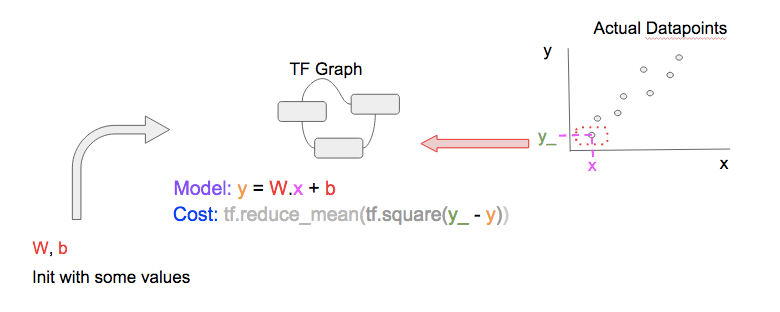
Our linear model and cost function equations [A] can be represented as TF graph as shown:

Next, we select a datapoint (x, y_) [C], and feed [D] it into the TF Graph to get the prediction (y) as well as the cost.

To get better W, b, we perform gradient descent using TF’stf.train.GradientDescentOptimizer [B] to reduce the cost. In non-technical terms: given the current cost, and based on the graph of how cost varies with other variables (namely W, b), the optimizer will perform small tweaks (increments/decrements) to W, b so that our prediction becomes better forthat single datapoint.

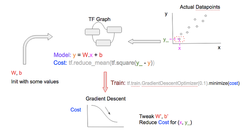
The final step in the training cycle is to update the W, b after tweaking them. Note that ‘cycle’ is also referred to as ‘epoch’ in ML literature.

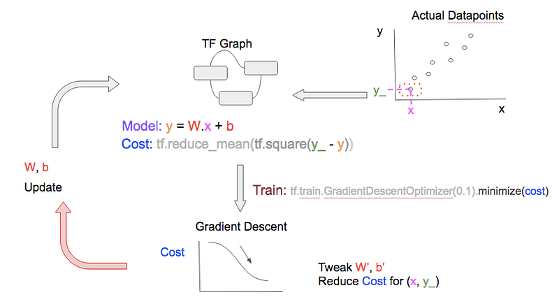
In the next training epoch, repeat the steps, but use a different datapoint!

Using a variety of datapoints generalizes our model, i.e., it learns W, b values that can be used to predict any feature value. Note that:

• In most cases, the more datapoints, the better your model can learn and generalize
• If you train more epochs than datapoints you have, you can re-use datapoints, which is not an issue. The gradient descent optimizer always use both the datapoint, AND the cost (calculated from the datapoint, with W, b values of that epoch) to tweak W, b; the optimizer may have seen that datapoint before, but not with the same cost, thus it will learn something new, and tweak W, b differently.

You can train the model a fixed number of epochs or until it reaches a cost threshold that is satisfactory.