The “Hello World” of Tensorflow
In this article, we will build a beginner-friendly machine learning model using TensorFlow.
Tensorflow is an open-source end-to-end machine learning framework that makes it easy to train and deploy the model.
It consists of two words - tensor and flow. A tensor is a vector or a multidimensional array that is a standard way of representing the data in deep learning models. Flow implies how the data moves through a graph by undergoing the operations called nodes.
It is used for numerical computation and large-scale machine learning by bundling various algorithms together. Besides, it also allows the flexibility and control to build models with high-level Keras API.
In this article, we will build a beginner-friendly machine learning model using TensorFlow.
We will be using credit card fraud detection data sourced from Kaggle.
The article is structured as follows:
- Understand the problem statement
- Load the data and required libraries
- Understand the data and evaluation metric for model selection
- Missing values
- Data Transformation
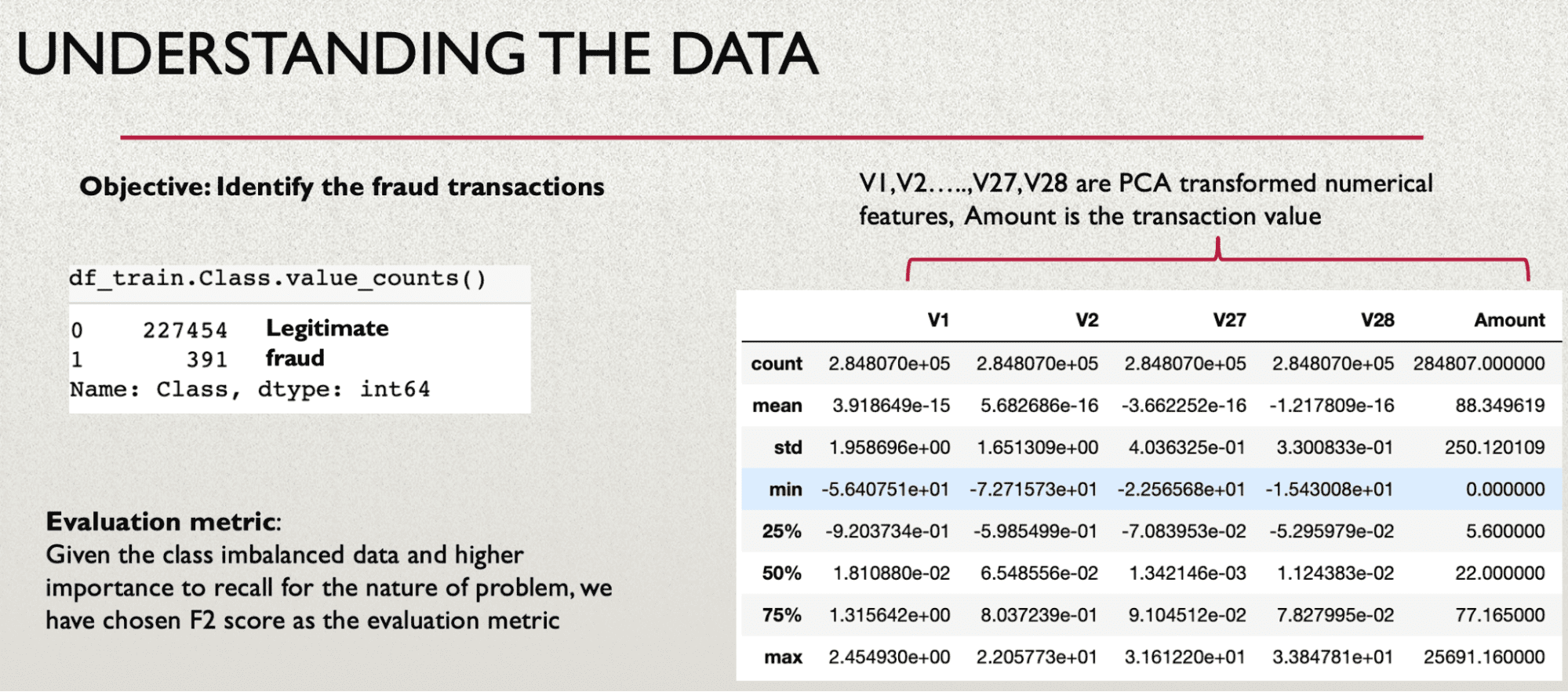
- Check the class imbalance
- Build TensorFlow model with class imbalance
- Evaluate the model performance
- Handle class imbalance and train the model
- Compare model performance with and without class imbalance
Problem Statement
Credit card transactions are subject to the risk of fraud i.e. those transactions are made without the knowledge of the customer. Machine learning models are deployed at various credit card companies to identify and flag potentially fraudulent transactions and timely act on them.
Load Data and Required Libraries
We have made two imports from TensorFlow:
- Dense layers where each neuron from the current layer is connected with all the neurons from the previous layer
- Another import is the Sequential model which is used to build the neural network.
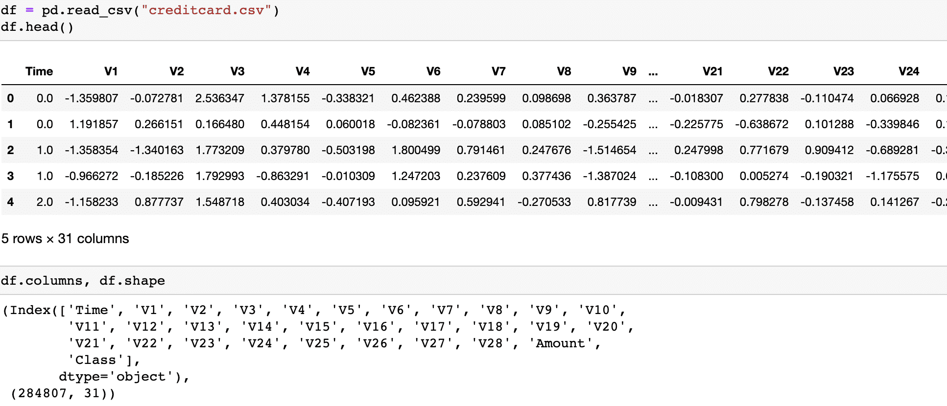
Get the Data
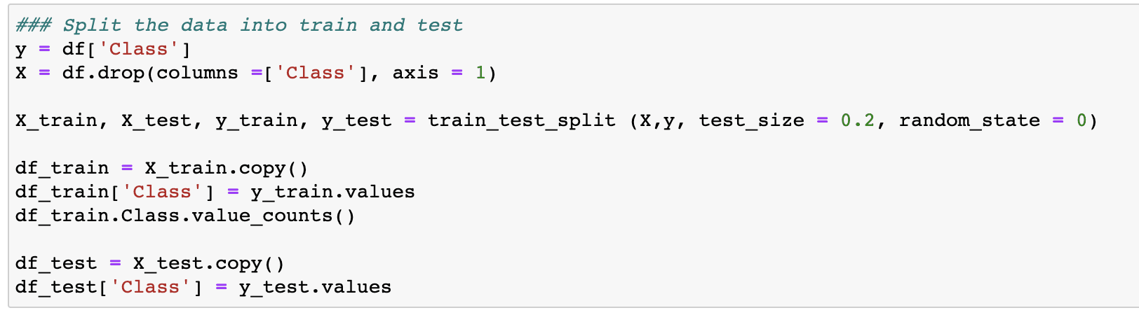
Splitting Into Train and Test Data
We have kept 20% of the data for evaluating the model performance and would start exploring the train data. Test data will be prepared in the same way as the train data along with all the transformations.
Understanding the Data
The data consists of PCA transformed numerical input variables that are masked, hence there is limited scope in understanding the attributes from business prerogative.
We have used tensorflow data validation library to visualize the attributes, it helps in understanding the training and the test data by computing descriptive statistics and detecting anomalies.
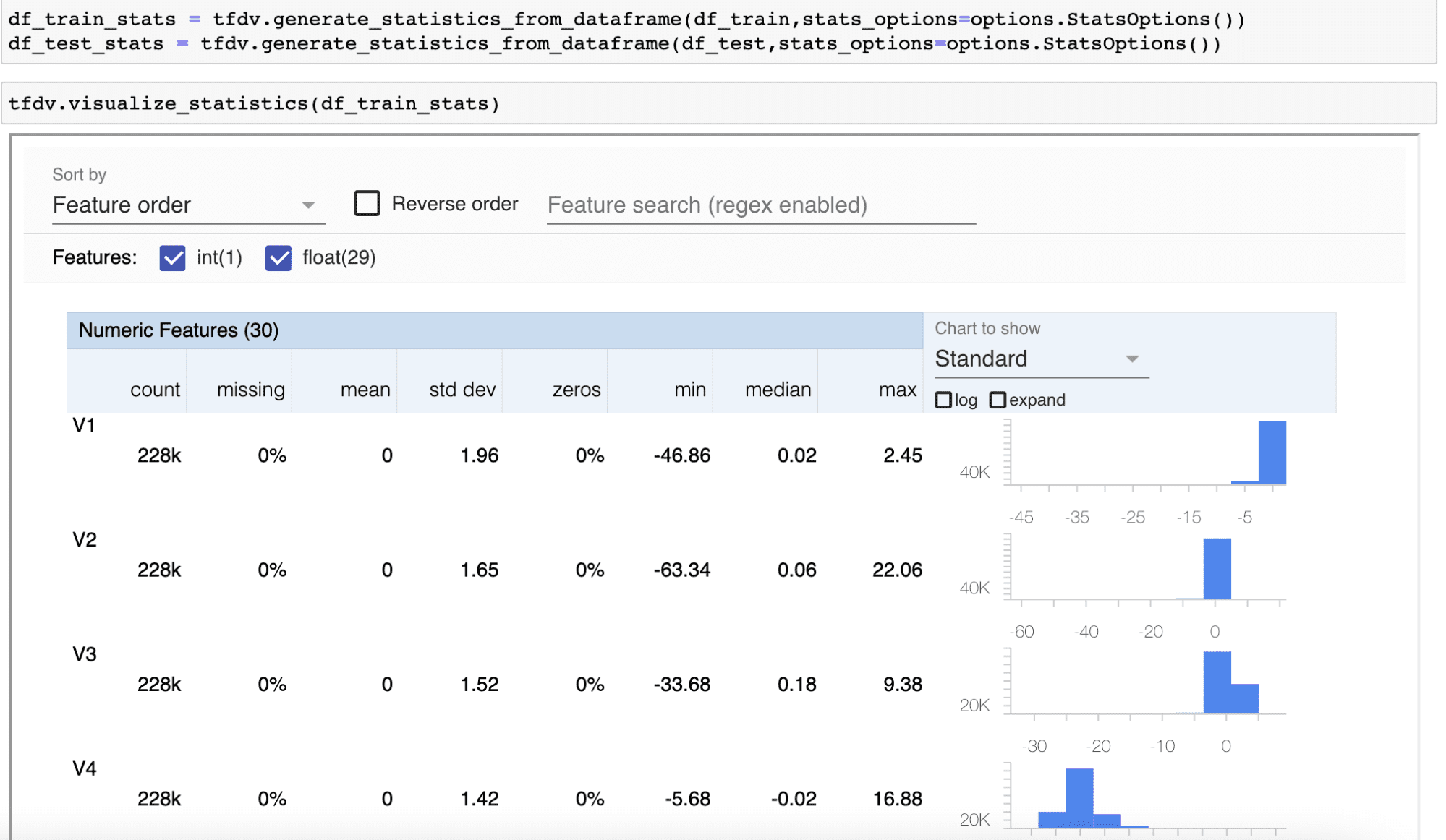
Besides, the attributes do not have any missing value and are PCA transformed, hence we are not performing any data transformation on these attributes. In the above visualization, you also have an option of performing log transformation to visualize the transformed data distribution.
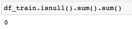
Missing Data
There is no missing value in any of the attributes as shown in the missing column in the above image, you can also do a quick check to sum all the null values across the attributes as below:
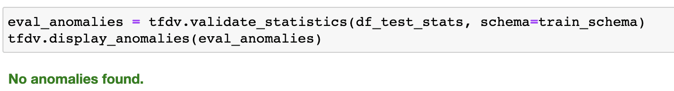
Train and Test Characteristics
One of the most critical assumptions in ML data modeling is that train and test dataset belong to similar distribution, as is evident from graphs below. The degree of the overlap between the train and test data distribution gives confidence that the trained model will be able to generalize well on the test data. It is important to keep monitoring if the serving data distribution deviates from the data on which the machine learning model was trained. You can then decide when to retrain the model with what partition of data.

You can also check out of domain value and detect errors or anomalies:
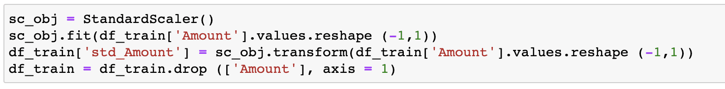
Data Transformation
As all the attributes except ‘Amount’ are PCA transformed, we will focus on ‘Amount’ and standardize it as below:
Preparing the Test Data
We will prepare the test data by applying the same transformations as were done on the training data:
Build the Baseline TensorFlow Model
Besides the units of neurons and the type of activation function, the first layer needs an additional input in the form of a number of input variables. The first two layers have ReLU activation which is a nonlinear function, you can read more on it here. We need the output as the probability of which class the transaction belongs to, hence the sigmoid activation function is chosen in the last layer.
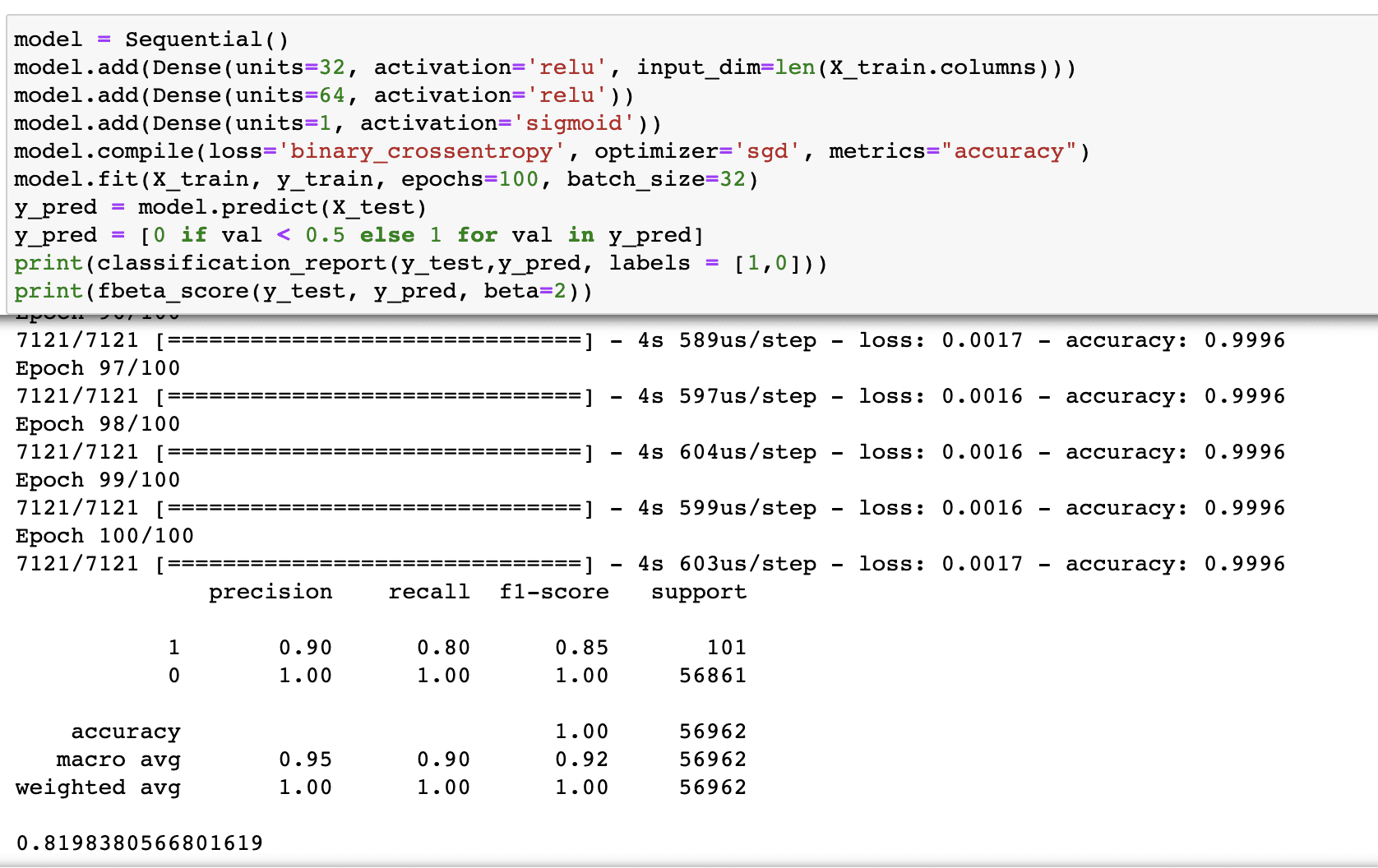
Evaluation Metric
Our objective is to reduce the false negatives, that is if the model declares a transaction as non-fraud and legitimate and it turns out to be false, then the whole purpose of building the model gets defeated. The model has passed through the fraudulent transaction which is worse than flagging the legitimate transaction as fraud.
Let's see what cost the ecosystem pays for the False Positives: If the customer makes a genuine transaction but due to a high false-positive rate, the model falsely claims this to be a fraud, and the transaction is declined. The customer has to go through additional authentication steps to confirm that he/she has triggered it. This hassle is also a cost but is less than the cost of letting the fraud pass through. Having said that, the good model can not block every transaction making it a pain for the genuine customers - hence a certain degree of precision is also important.
F1 is the harmonic mean of precision and recall. Depending upon which one is more important for the business metric, one can be given more weight than the other. This can be achieved by fbeta_score which is the weighted harmonic mean of precision and recall, where beta is the weight of recall in the combined score.
| beta < 1 | more weight to precision |
| beta < 1 | more weight to recall |
| beta = 0 | considers only precision |
| beta = inf | considers only recall |
Hence, for the purpose of this article, we are using an F2 score that gives twice the weightage to recall.
Handling the Class Imbalance
We have downsampled the majority class by taking a random sample of 10% and concatenating it back with the minority class i.e. fraud transactions.
Note that we have separated the train and test data before, and kept the test data aside to compare the model output from both the versions i.e. trained with and without class imbalance handling.
A Model Trained with Class Imbalance Handled
The new model is trained on data distribution as shown below:
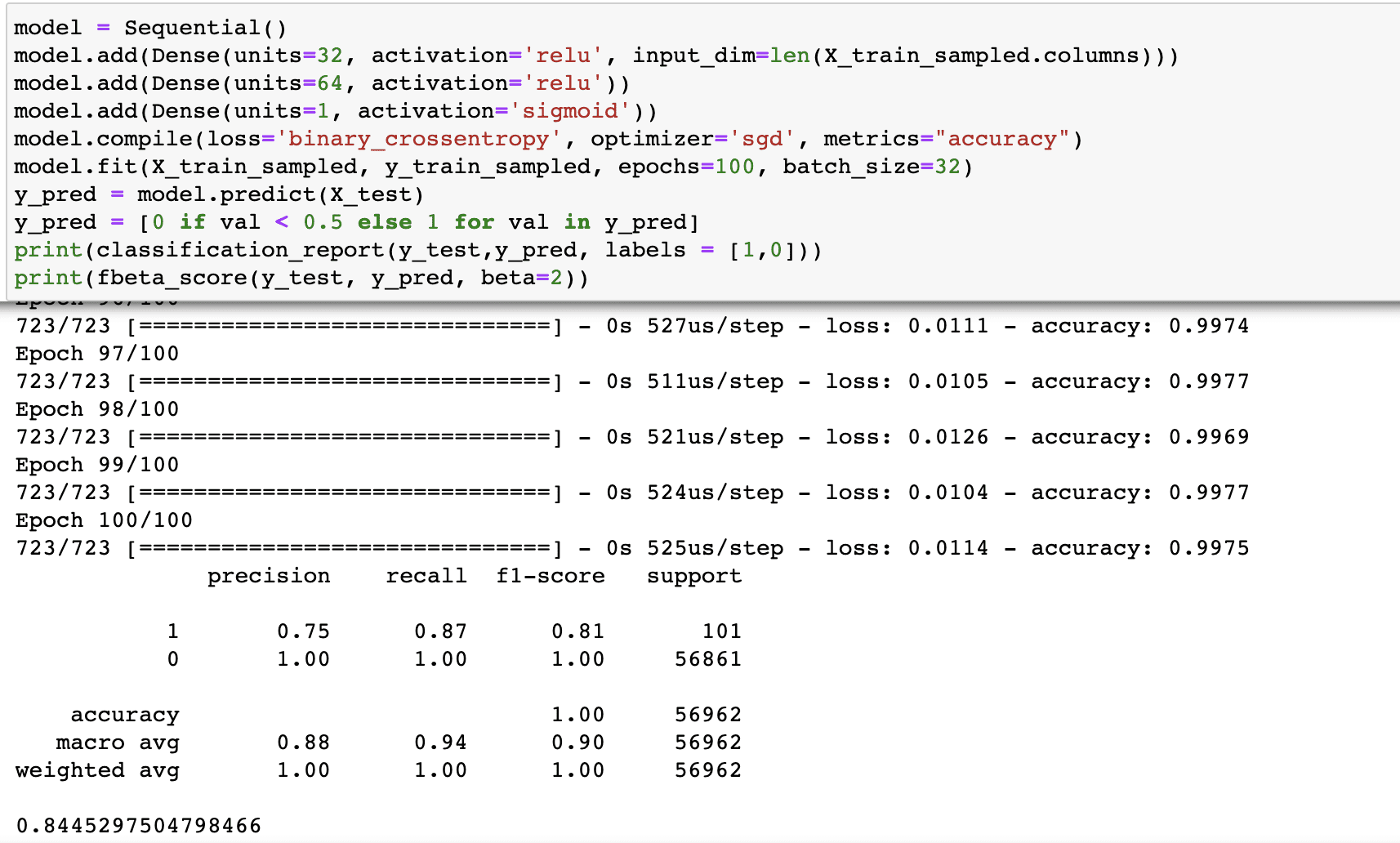
As we can see above, the recall has increased from 80% to 87% for class 1, albeit at the cost of a decline in precision. Also, the F2 score has increased from 82% to 84.5% in the revised model trained with improved class-balanced data distribution.
Note that you can adjust the cut-off to achieve the target recall and precision values.
In this article, we have built a neural network model to identify fraudulent transactions. Since the dataset is imbalanced, we have undersampled the majority class to improve the class distribution. This has resulted in improved recall value (primary metric) for the concerned class i.e. class 1 and improved F2 score.
Vidhi Chugh is an award-winning AI/ML innovation leader and an AI Ethicist. She works at the intersection of data science, product, and research to deliver business value and insights. She is an advocate for data-centric science and a leading expert in data governance with a vision to build trustworthy AI solutions.