Image by Author

AI has gone so far now, and various state-of-the AI models are evolving that are used in Chatbots, Humanoid Robots, Self-driving cars, etc. It has become the fastest-growing technology, and Object Detection and Object Classification are trendy these days.

In this blog post, we will cover the complete steps of building and training an Image Classification model from scratch using Convolutional Neural Network. We will use the publicly available Cifar-10 dataset to train the model. This dataset is unique because it contains images of everyday seen objects like cars, aeroplanes, dogs, cats, etc. By training the neural network to these objects, we will develop intelligent systems to classify such things in the real world. It contains more than 60000 images of size 32x32 of 10 different types of objects. By the end of this tutorial, you will have a model which can determine the object based on its visual features.

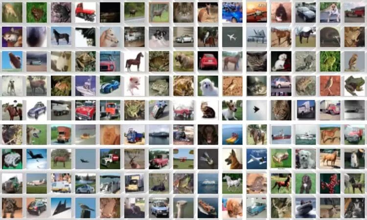
Fig. 1 Sample Images of the Dataset | Image by datasets.activeloop

We will cover everything from scratch, so if you have yet to learn about the practical implementation of neural networks, it is completely fine. The only prerequisite of this tutorial is your time and the basic knowledge of Python. At the end of this tutorial, I will share the collaboratory file containing the entire code. Let’s get started!

Here is the complete workflow of this tutorial,

1. Importing Necessary Libraries
2. Loading of the Data
3. Preprocessing of the Data
4. Building the Model
5. Evaluating the Model Performance

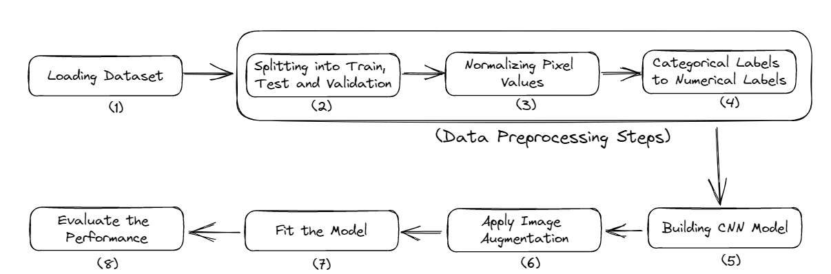
Fig. 2 Complete Model Pipeline | Image by Author

Importing Necessary Libraries

You have to install some modules to start with the project. I will use Google Colab as it provides free GPU training, and at the end, I will provide you with the collaboratory file containing the complete code.

Here is the command to install the required libraries:

$ pip install tensorflow, numpy, keras, sklearn, matplotlib

Importing the libraries into a Python file.

from numpy import *
from pandas import *
import matplotlib.pyplot as plotter

# Split the data into training and testing sets.
from sklearn.model_selection import train_test_split

# Libraries used to evaluate our trained model.
from sklearn.metrics import classification_report, confusion_matrix
import keras

# Loading our dataset.
from keras.datasets import cifar10

# Used for data augmentation.
from keras.preprocessing.image import ImageDataGenerator

# Below are some layers used to train convolutional nueral network.
from keras.models import Sequential
from keras.layers import Dense, Dropout, Activation
from keras.layers import Conv2D, MaxPooling2D, GlobalMaxPooling2D, Flatten

1. Numpy: It is used for efficient array computations of large datasets containing images.
2. Tensorflow: It is an open-source machine learning library developed by Google. It provides numerous functions to build large and scalable models.
3. Keras: Another high-level neural network API runs on top of TensorFlow.
4. Matplotlib: This Python library creates plots and graphs, providing better data visualisation.
5. Sklearn: It provides functions for performing data preprocessing and feature extraction tasks for the dataset. It contains inbuilt functions to find the evaluation metrics of a model like accuracy, precision, false positives, false negatives, etc.

Now, let's move to the step of data loading.

Loading the Data

This section will load our dataset and performs the train-test splitting.

Loading & Splitting of Data:

# number of classes
nc = 10

(training_data, training_label), (testing_data, testing_label) = cifar10.load_data()
(
    (training_data),
    (validation_data),
    (training_label),
    (validation_label),
) = train_test_split(training_data, training_label, test_size=0.2, random_state=42)
training_data = training_data.astype("float32")
testing_data = testing_data.astype("float32")
validation_data = validation_data.astype("float32")

The cifar10 dataset is directly loaded from the Keras datasets library. And this data is also split into training data and testing data. Training data is used to train the model so that it can identify patterns in it. And the testing data remain unseen to the model, and it is used to check its performance, i.e. how many data points are correctly predicted wrt the total data points.

training_label contains the corresponding label to the image present in training_data.

Then the training data is again split into the validation data using the built-in sklearn train_test_split function. The validation data is used to select and tune the final model. Then finally, all the training, testing and validation data are converted into floating decimals of 32bit.

Now, the loading of our dataset is done. In the next section, we will perform some preprocessing steps to it.

Pre-processing of Data

Data preprocessing is the first and most crucial step while developing a machine learning model. Let's see how to do it.

# Normalization
training_data /= 255
testing_data /= 255
validation_data /= 255

# One Hot Encoding
training_label = keras.utils.to_categorical(training_label, nc)
testing_label = keras.utils.to_categorical(testing_label, nc)
validation_label = keras.utils.to_categorical(validation_label, nc)

# Printing the dataset
print("Training: ", training_data.shape, len(training_label))
print("Validation: ", validation_data.shape, len(validation_label))
print("Testing: ", testing_data.shape, len(testing_label))

Output:

Training:  (40000, 32, 32, 3) 40000
Validation:  (10000, 32, 32, 3) 10000
Testing:  (10000, 32, 32, 3) 10000

The dataset contains images of 10 classes, and the size of each image is 32x32 pixels. Each pixel has a value from 0-255, and we need to normalise it between 0-1 to ease the calculation process. And after that, we will convert the categorical labels into the one-hot encoded labels. This is done to convert the categorical data into numerical data so we can apply machine learning algorithms without any problem.

Now, move to the building of the CNN model.

Building the CNN Model

The CNN Model works in 3 stages. The first stage consists of convolutional layers that extract relevant features from the images. The second stage consists of pooling layers used to reduce the dimensionality of the images. It also helps to reduce the overfitting of the model. And the third stage consists of dense layers that convert the two-dimensional image to a one-dimensional array. And then finally, this array is fed onto the fully connected layers, which perform the final prediction.

Here is the code.

model = Sequential()

model.add(
    Conv2D(32, (3, 3), padding="same", activation="relu", input_shape=(32, 32, 3))
)
model.add(Conv2D(32, (3, 3), padding="same", activation="relu"))
model.add(MaxPooling2D((2, 2)))
model.add(Dropout(0.25))

model.add(Conv2D(64, (3, 3), padding="same", activation="relu"))
model.add(Conv2D(64, (3, 3), padding="same", activation="relu"))
model.add(MaxPooling2D((2, 2)))
model.add(Dropout(0.25))

model.add(Conv2D(96, (3, 3), padding="same", activation="relu"))
model.add(Conv2D(96, (3, 3), padding="same", activation="relu"))
model.add(MaxPooling2D((2, 2)))

model.add(Flatten())
model.add(Dropout(0.4))
model.add(Dense(256, activation="relu"))
model.add(Dropout(0.4))
model.add(Dense(128, activation="relu"))
model.add(Dropout(0.4))
model.add(Dense(nc, activation="softmax"))

We have applied the three sets of layers, each containing two convolutional layers, one max-pooling layer and one dropout layer. The Conv2D layer takes the input_shape as (32, 32, 3), which must be the same as the dimensions of the image.

Each Conv2D layer also takes an activation function, i.e. ‘relu’. Activation functions are used to increase the non-linearity in the system. In simpler terms, it decides whether the neuron needs to be activated or not based on a certain threshold. There are many types of activation functions like ‘ReLu’, ‘Tanh’, ‘Sigmoid’, ‘Softmax’, etc., which use different algorithms to decide the firing of the neuron.

After that, the Flattening Layer and the Fully Connected Layers are added, with several Dropout layers in between them. The dropout layer rejects some of the neurons' contribution towards the net layer randomly. The parameter inside it defines the degree of rejection. It is mainly used to avoid over-fitting.

Below is a sample image of what a CNN model architecture looks like.

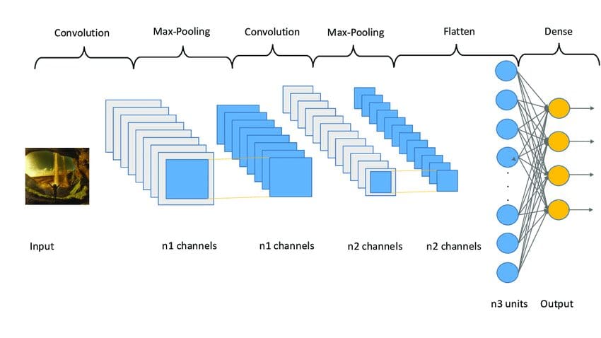
Fig. 3 Sampe CNN Architecture | Image by researchgate

Compiling the Model

Now, we will compile and prepare the model for the training.

# initiate Adam optimizer
opt = keras.optimizers.Adam(lr=0.0001)

model.compile(loss="categorical_crossentropy", optimizer=opt, metrics=["accuracy"])
# obtaining the summary of the model
model.summary()

Output:

Fig. 4 Model Summary | Image by Author

We have used the Adam optimizer with a learning rate of 0.0001. Optimizer decides how the model's behaviour changes in response to the output of the loss function. The Learning Rate is the amount of weights updated during training or the step size. It is a configurable hyperparameter that must not be too small or too large.

Fitting the Model

Now, we will fit the model to our training data and start the training process. But before that, we will use Image Augmentation to increase the number of sample images.

Image Augmentation used in Convolutional Neural Networks will increase the training images without requiring new images. It will replicate the images by producing some amount of variation in it. It can be done by rotating the image to some degree, adding noise, flipping it horizontally or vertically, etc.

augmentor = ImageDataGenerator(
    width_shift_range=0.4,
    height_shift_range=0.4,
    horizontal_flip=False,
    vertical_flip=True,
)

# fitting in augmentor
augmentor.fit(training_data)

# obtaining the history
history = model.fit(
    augmentor.flow(training_data, training_label, batch_size=32),
    epochs=100,
    validation_data=(validation_data, validation_label),
)

Output:

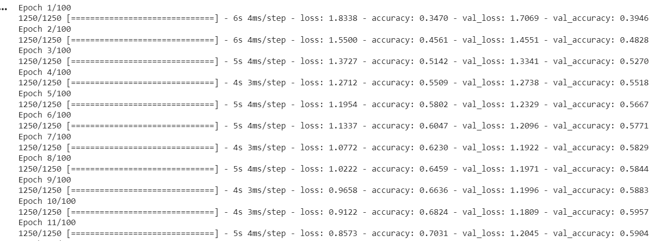
Fig.5 Accuracy & Loss at each Epoch | Image by Author

ImageDataGenerator() function is used to create augmented images. The fit() is used to fit the model. It takes the training and validation data, Batch Size, and the number of Epochs as input

Batch Size is the number of samples processed before the model gets updated. A crucial hyperparameter must be greater than equal to one and less than equal to the number of samples. Usually, 32 or 64 are considered the best Batch Sizes.

The number of Epochs represents how many times all the samples are processed once individually on both the forward and backward to the network. 100 epochs mean the whole dataset passes through the model 100 times, and the model runs 100 times itself.

Our model is trained, and now we will evaluate its performance on the test set.

Evaluating Model Performance

In this section, we will check the accuracy and loss of the model on the test set. Also, we will draw a plot between the Accuracy Vs Epoch and Loss Vs Epoch for training and validation data.

model.evaluate(testing_data, testing_label)

Output:

313/313 [==============================] - 2s 5ms/step - loss: 0.8554 - accuracy: 0.7545
[0.8554493188858032, 0.7545000195503235]

Our model achieved an accuracy of 75.34% with a loss of 0.8554. This accuracy can be increased as this is not a state-of-the-art model. I used this model to explain the process and flow of building a model. The accuracy of the CNN model depends on many factors like choice of layers, selection of hyperparameters, the type of dataset used, etc.

Now we will plot the curves to check overfitting in the model.

def acc_loss_curves(result, epochs):
    acc = result.history["accuracy"]
    # obtaining loss and accuracy
    loss = result.history["loss"]
    # declaring values of loss and accuracy
    val_acc = result.history["val_accuracy"]
    val_loss = result.history["val_loss"]
    # plotting the figure
    plotter.figure(figsize=(15, 5))
    plotter.subplot(121)
    plotter.plot(range(1, epochs), acc[1:], label="Train_acc")
    plotter.plot(range(1, epochs), val_acc[1:], label="Val_acc")
    # giving title to plot
    plotter.title("Accuracy over " + str(epochs) + " Epochs", size=15)
    plotter.legend()
    plotter.grid(True)
    # passing value 122
    plotter.subplot(122)
    # using train loss
    plotter.plot(range(1, epochs), loss[1:], label="Train_loss")
    plotter.plot(range(1, epochs), val_loss[1:], label="Val_loss")
    # using ephocs
    plotter.title("Loss over " + str(epochs) + " Epochs", size=15)
    plotter.legend()
    # passing true values
    plotter.grid(True)
    # printing the graph
    plotter.show()


acc_loss_curves(history, 100)

Output:

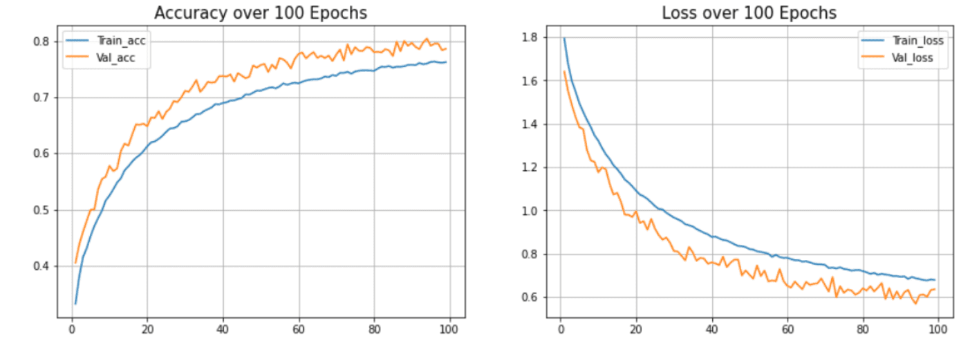
Fig.6 Accuracy and Loss Vs Epoch | Image by Author

In our model, we can see that the model overfits the test dataset. The (blue) line indicates the training accuracy, and the (orange) line indicates the validation accuracy. The training accuracy continues improving, but the validation error worsens after 20 epochs.

Please find the Google Colab link used in this article - Link

Conclusion

This article shows the entire process of building and training a Convolutional Neural Network from scratch.  We got around 75% accuracy. You can play with the hyperparameters and use different sets of convolutional and pooling layers to improve the accuracy. You can also try Transfer Learning, which uses pre-trained models like ResNet or VGGNet and gives very good accuracy in some cases. We can talk more about it in other articles if you want.

Until then, keep reading and keep learning. Feel free to contact me on Linkedin in case of any questions or suggestions.
 
 
Aryan Garg is a B.Tech. Electrical Engineering student, currently in the final year of his undergrad. His interest lies in the field of Web Development and Machine Learning. He have pursued this interest and am eager to work more in these directions.