K-Nearest Neighbors – the Laziest Machine Learning Technique

By Rapidminer Sponsored Post.

K-Nearest Neighbors (K-NN) is one of the simplest machine learning algorithms. Like other machine learning techniques, it was inspired by human reasoning. For example, when something significant happens in your life, you memorize that experience and use it as a guideline for future decisions.

Let me give you a scenario of a person dropping a glass. While the glass is falling, you’ve made the prediction that the glass will break when it hits the ground. But how can you do this? You never have seen this glass break before, right?

No, indeed not. But, you have seen similar glasses drop to the floor before. And while the situation might not be exactly the same, you know that a glass dropping from 5-feet onto a concrete floor usually breaks, giving you a high level of confidence that will be the outcome.

But what about dropping a glass from a short distance onto a soft carpet? Have you experienced this as well? We can see that the distance and ground surface both play a role in the outcome.

This is the same reasoning the K-NN algorithm is using. When a new situation occurs, it scans through all past experiences and looks up the k closest experiences. Those experiences (or: data points) are what we call the k nearest neighbors.

If you have a classification task, for example you want to predict if the glass will break, you take the majority vote of all k neighbors.  If k=5 and in 3 or more of your most similar experiences the glass broke, it will go with the prediction “yes, it will break”.

Let’s now assume that you want to predict the number of pieces a glass will break into. In this case, you want to predict a number which we call “regression”.  You take the average value of your k neighbors’ numbers of glass pieces as a prediction or score. If k=5 and the numbers of pieces are 1 (did not break), 4, 8, 2, and 10 you will end up with the prediction of 5.

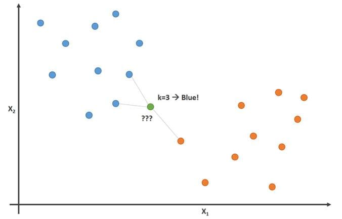
We have blue and orange data points.  For a new data point (green), we can determine the most likely class by looking up the classes of the nearest neighbors.  Here, the decision would be “blue”, because that is the majority of the neighbors.

So why is this algorithm “lazy”? That’s because it doesn’t do any training when you supply the training data. At training time, all it is doing is storing the data set. It doesn’t do any calculations at this point. Nor does it try to derive a more compact model from the data which it could use for scoring.  

 

Theory

 
All the computation happens during scoring, i.e. when you apply the model on unseen data points. You need to determine which k data points out of our training set are closest to the data point we want to get a prediction for.

Let’s say that our data points look like the following:

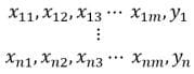
We have a table of n rows and m+1 columns where the first m columns are the attributes we use to predict the remaining label column (also known as “target”). For now, let’s also assume that all attribute values x are numerical, while the label values for y are categorical, i.e. we have a classification problem.

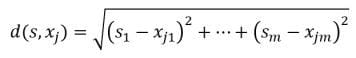
We can now define a distance function which calculates the distance between data points. It should find the closest data points from our training data for any new point. The Euclidean distance is often a good choice for a distance function if the data is numerical. If our new data point has attribute values s1 to sm, we can calculate the distance d(s, xj) between point s to any data point xj by

The k data points with the closest value for this distance become our k neighbors. For a classification task, we now use the most frequent of all values yfrom our k neighbors. For regression tasks, where y is numerical, we use the average of all values y from our k neighbors.

But what if our attributes are not numerical and don’t consist of numerical and categorical attributes? Then you can use any other distance measure which can handle this type of data.  This article discusses some frequent choices.

By the way, K-NN models with k=1 are the reason why calculating training errors are completely pointless.  Can you see why?

 

Practical Usage

 
K-NN should be a standard tool in your toolbox. It is fast, easy to understand, and easy to tune to different kinds of predictive problems.

Data Preparation

There are some things to consider with K-NN. We have seen that the key part of the algorithm is the definition of a distance measure, and the Euclidean distance is often used. This distance measure treats all data columns in the same way though. It subtracts the values for each dimension before it sums up the squares of those distances. And that means that columns with a wider data range have a larger influence on the distance than columns with a smaller data range.

So, you need to normalize the data set so that all columns are roughly on the same scale. There are two common ways of normalization. First, you could bring all values of a column into a range between 0 and 1. Or you could change the values of each column so that the column has a mean 0 with a standard deviation of 1 afterwards. We call this type of normalization z-transformation or standard score.

Tip: Whenever you know that the machine learning algorithm is making use of a distance measure, you should normalize the data. Another famous example would be k-Means clustering.

Parameters to Tune

The most important parameter you need to tune is k, the number of neighbors used to make the class decision. The minimum value is 1 in which case you only look at the closest neighbor for each prediction to make your decision. In theory, you could use a value for k which is as large as your total training set. This would make no sense though, since in this case you would always predict the majority class of the complete training set.

Here is a good way to interpret the meaning behind k. Small numbers indicate “local” models, which can be non-linear and the decision boundary between the classes wiggle a lot. If the number grows, the wiggling gets less until you almost end up with a linear decision boundary.

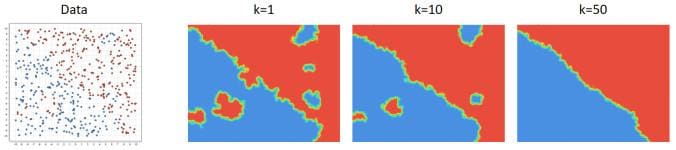
We see a data set in two dimensions on the left.  In general, the top right is red and the bottom left is the blue class.  But there are also some local groups inside of both areas.  Small values for k lead to more wiggly decision boundaries.  For larger values the decision boundary becomes smoother, almost linear in this case.

Good values for k depend on the data you have and if the problem is non-linear. You should try a couple of values between 1 and about 10% of the size of the training data set size to see if there is a promising area worth the further optimization of k.

The second parameter you might want to consider is the type of distance function you are using.  For numerical values, Euclidean distance is a good choice.  You might want to try Manhattan distance which is sometimes used as well.  For text analytics, cosine distance can be another good alternative worth trying.

Memory Usage & Runtimes

Please note that all this algorithm is doing is storing the complete training data.  So, the memory needs grow linearly with the number of data points you provide for training.  Smarter implementations of this algorithm might choose to store the data in a more compact fashion. But in a worst-case scenario you still end up with a lot of memory usage.

For training, the runtime is as good as it gets.  The algorithm is doing no calculations at all besides storing the data which is fast.

The runtime for scoring though can be large though which is unusual in the world of machine learning.  All calculations happen during model application. Hence, the scoring runtime scales linearly with the number of data columns m and the number of training points n. If you need to score fast and the number of training data points is large, then K-NN is not a good choice.

RapidMiner Processes

Want to build this machine learning model yourself? Download RapidMiner and use the processes below*.

• Train and apply a K-NN model: knn_training_scoring
• Optimize the value for k: knn_optimize_parameter

*Download the Zip-file and extract its content.  The result will be an .rmp file which can be loaded into RapidMiner via “File” -> “Import Process”.