Another day, another classic algorithm: k-nearest neighbors. Like the naive Bayes classifier, it’s a rather simple method to solve classification problems. The algorithm is intuitive and has an unbeatable training time, which makes it a great candidate to learn when you just start off your machine learning career. Having said this, making predictions is painfully slow, especially for large datasets. The performance for datasets with many features might also not be overwhelming, due to the curse of dimensionality.

In this article, you will learn

• how the k-nearest neighbors classifier works
• why it was designed like this
• why it has these severe disadvantages and, of course,
• how to implement it in Python using NumPy.

As we will implement the classifier in a scikit learn-conform way, it’s also worthwhile to check out my article Build your own custom scikit-learn Regression. However, the scikit-learn overhead is quite small and you should be able to follow along anyway.

You can find the code on my Github.

Theory

The main idea of this classifier is stunningly simple. It is directly derived from the fundamental question of classifying:

Given a data point x, what is the probability of x belonging to some class c?

In the language of mathematics, we search for the conditional probability p(c|x). While the naive Bayes classifier tries to model this probability directly using some assumptions, there is another intuitive way to compute this probability — the frequentist view of probability.

The naive View on Probabilities

Ok, but what does this mean now? Let us consider the following simple example: You roll a six-sided, possibly rigged die and want to compute the probability of rolling a six, i.e. p(roll number 6). How to do this? Well, you roll the die n times and write down how often it showed a six. If you have seen the number six k times, you say the probability of seeing a six is around k/n. Nothing new or fancy here, right?

Now, imagine that we want to compute a conditional probability, for example

p(roll number 6 | roll an even number)

You don’t need Bayes’ theorem to solve this. Just roll the die again and ignore all the rolls with an odd number. That’s what conditioning does: filtering results. If you rolled the die n times, have seen m even numbers and k of them were a six, the probability above is around k/m instead of k/n.

Motivating k-Nearest Neighbors

Back to our problem. We want to compute p(c|x) where x is a vector containing the features and c is some class. As in the die example, we

• need a lot of data points,
• filter out the ones with features x and
• check how often these data points belong to class c.

The relative frequency is our guess for the probability p(c|x).

Do you see the problem here?

Usually, we don’t have many data points with the same features. Often only one, maybe two. For example, imagine a dataset with two features: the height (in cm) and the weight (in kg) of persons. The labels are male or female. Thus, x=(x?, x?) where x? is the height and x? is the weight, and c can take the values male and female. Let us look at some dummy data:

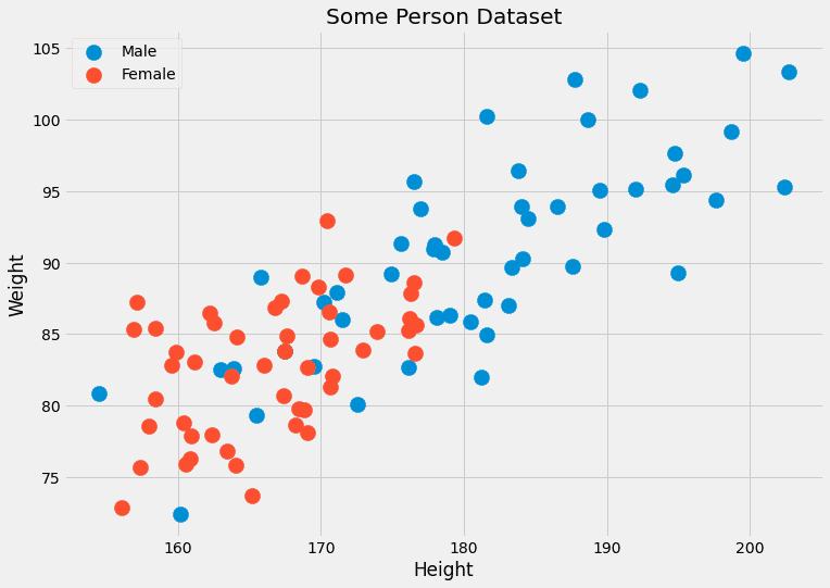
Image by the Author.

Since these two features are continuous, the probability of having two, let alone several hundred, data points is negligible.

Another problem: what happens if we want to predict the gender for a data point with features we have never seen before, such as (190.1, 85.2)? That is what prediction is actually all about. That’s why this naive approach does not work. What the k-nearest neighbor algorithm does instead is the following:

It tries to approximate the probability p(c|x) not with data points that have exactly the features x, but with data points with features close to x.

It is less strict, in a sense. Instead of waiting for a lot of persons with height=182.4 and weight=92.6, and checking their gender, k-nearest neighbors allows considering people close to having these characteristics. The k in the algorithm is the number of people we consider, it is a hyperparameter.

These are parameters that we or a hyperparameter optimization algorithm such as grid search have to choose. They are not directly optimized by the learning algorithm.

Image by the Author.

The Algorithm

We have everything we need now to describe the algorithm.

Training:

1. Organize the training data in some way. During prediction time, this order should make it possible to give us the k closest points for any given data point x.
2. That’s it already! ????

Prediction:

1. For a new data point x, find the k closest neighbors in the organized training data.
2. Aggregate the labels of these k neighbors.
3. Output the label/probabilities.

We can’t implement this so far, because there are a lot of blanks we have to fill in.

• What does organizing mean?
• How do we measure proximity?
• How to aggregate?

Besides the value for k, these are all things we can choose, and different decisions give us different algorithms. Let’s make it easy and answer the questions as follows:

• Organizing = just save the training dataset as it is
• Proximity = Euclidean distance
• Aggregation = Averaging

This calls for an example. Let us check the picture with the person data again.

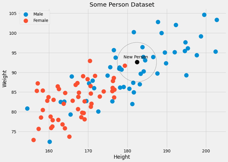
We can see that the k=5 closest data points to the black one have 4 male labels and one female label. So we could output that the person belonging to the black point is, in fact, 4/5=80% male and 1/5=20% female. If we prefer a single class as output, we would return male. No problem!

Now, let us implement it.

Implementation

The hardest part is to find the nearest neighbors to a point.

A quick primer

Let us do a small example of how you can do this in Python. We start with

import numpy as np

features = np.array([[1, 2], [3, 4], [1, 3], [0, 2]])
labels = np.array([0, 0, 1, 1])

new_point = np.array([1, 4])

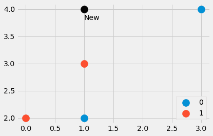
Image by the Author.

We have created a small dataset consisting of four data points, as well as another point. Which are the closest points? And should the new point have the label 0 or 1? Let us find out. Typing in

distances = ((features - new_point)**2).sum(axis=1)

gives us the four values distances=[4, 4, 1, 5], which is the squared Euclidean distance from new_point to all other points in features . Sweet! We can see that point number three is the closest, followed by points number one and two. The fourth point is furthest away.

How can we extract the closest points now from the array [4, 4, 1, 5]? A distances.argsort() helps. The result is [2, 0, 1, 3] which tells us that the data point with index 2 is the smallest (out point number three), then the point with index 0, then with index 1, and finally the point with index 3 is the largest.

Note that argsort put the first 4 in distances before the second 4. Depending on the sorting algorithm, this could also be the other way around, but let’s not go into these details for this introductory article.

How if we want the three closest neighbors, for example, we could get them via

distances.argsort()[:3]

and the labels correspond to these closest points via

labels[distances.argsort()[:3]]

We get [1, 0, 0], where 1 is the label of the closest point to (1, 4), and the zeroes are the labels belonging to the next two closest points.

That’s all we need, let’s get to the real deal.

The final Code

You should be quite familiar with the code. The only new function is np.bincount which counts the occurrences of the labels. Note that I implemented a predict_proba method first to compute probabilities. The method predict just calls this method and returns the index (=class) with the highest probability using an argmaxfunction. The class awaits classes from 0 to C-1, where C is the number of classes.

Disclaimer: This code is not optimized, it only serves an educational purpose.

import numpy as np
from sklearn.base import BaseEstimator, ClassifierMixin
from sklearn.utils.validation import check_X_y, check_array, check_is_fitted

class KNNClassifier(BaseEstimator, ClassifierMixin):
    def __init__(self, k=3):
        self.k = k
    
    def fit(self, X, y):
        X, y = check_X_y(X, y)
        self.X_ = np.copy(X)
        self.y_ = np.copy(y)
        self.n_classes_ = self.y_.max() + 1
        
        return self
    
    def predict_proba(self, X):
        check_is_fitted(self)
        X = check_array(X)
        
        res = []
        for x in X:
            distances = ((self.X_ - x)**2).sum(axis=1)
            smallest_distances = distances.argsort()[:self.k]
            closest_labels = self.y_[smallest_distances]
            count_labels = np.bincount(
                closest_labels,
                minlength=self.n_classes_
            )
            
            res.append(count_labels / count_labels.sum())
        
        return np.array(res)
    
    def predict(self, X):
        check_is_fitted(self)
        X = check_array(X)
        
        res = self.predict_proba(X)
        
        return res.argmax(axis=1)

And that’s it! We can do a small test and see if it agrees with the scikit-learn k-nearest neighbor classifier.

Testing the Code

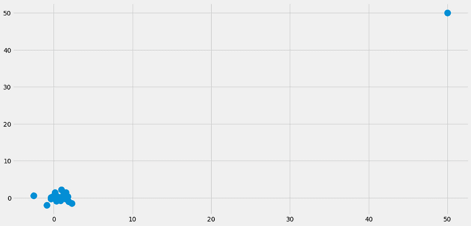
Let us create another small dataset for testing.

from sklearn.datasets import make_blobs
import numpy as np

X, y = make_blobs(n_samples=20, centers=[(0,0), (5,5), (-5, 5)], random_state=0)
X = np.vstack([X, np.array([[2, 4], [-1, 4], [1, 6]])])
y = np.append(y, [2, 1, 0])

It looks like this:

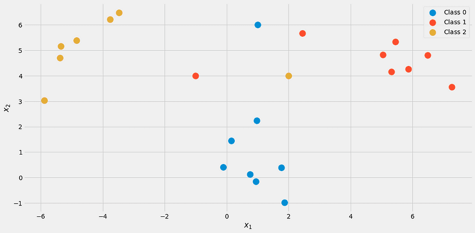
Image by the Author.

Using our classifier with k = 3

my_knn = KNNClassifier(k=3)
my_knn.fit(X, y)

my_knn.predict_proba([[0, 1], [0, 5], [3, 4]])

we get

array([[1.        , 0.        , 0.        ],
       [0.33333333, 0.33333333, 0.33333333],
       [0.        , 0.66666667, 0.33333333]])

Read the output as follows: The first point is 100% belonging to class 1 the second point lies in each class equally with 33%, and the third point is about 67% class 2 and 33% class 3.

If you want concrete labels, try

my_knn.predict([[0, 1], [0, 5], [3, 4]])

which outputs [0, 0, 1]. Note that in the case of a tie, the model as we implemented it outputs the lower class, that’s why the point (0, 5) gets classified as belonging to class 0.

If you check the picture, it makes sense. But let’s reassure ourselves with the help of scikit-learn.

from sklearn.neighbors import KNeighborsClassifier

knn = KNeighborsClassifier(n_neighbors=3)
knn.fit(X, y)

my_knn.predict_proba([[0, 1], [0, 5], [3, 4]])

The result:

array([[1.        , 0.        , 0.        ],
       [0.33333333, 0.33333333, 0.33333333],
       [0.        , 0.66666667, 0.33333333]])

Phew! Everything looks good. Let us check the decision boundaries of the algorithm, just because it’s pretty.

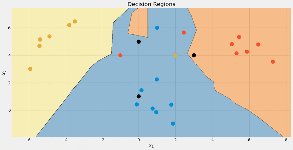
Image by the Author.

Again, the top black point is not 100% blue. It’s 33% blue, red and yellow, but the algorithm decides deterministically for the lowest class, which is blue.

We can also check the decision boundaries for different values of k.

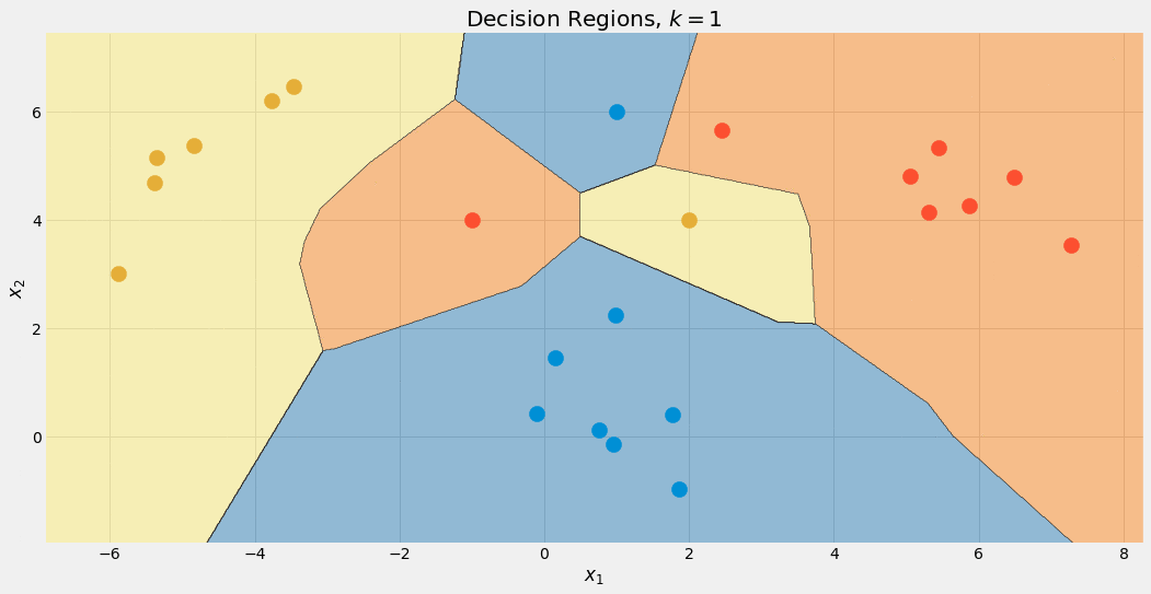
Image by the Author.

Note that the blue region gets bigger in the end, because of this preferential treatment of this class. We can also see that for k=1 the boundaries are a mess: the model is overfitting. On the other side of the extreme, k is as large as the size of the dataset, and all points are used for the aggregation step. Thus, each data point gets the same prediction: the majority class. The model is underfitting in this case. The sweet spot is somewhere in between and can be found using hyperparameter optimization techniques.

Before we get to the end, let us see which problems this algorithm has.

Drawbacks of k-Nearest Neighbors

The problems are as follows:

1. Finding the nearest neighbors takes a lot of time, especially with our naive implementation. If we want to predict the class of a new data point, we have to check it against every other point in our dataset, which is slow. There are better ways to organize the data using advanced data structures, but the problem still persists.
2. Following problem number 1: Usually, you train models on faster, stronger computers and can deploy the model on weaker machines afterward. Think about deep learning, for example. But for k-nearest neighbors, the training time is easy and the heavy work is done during prediction time, which is not what we want.
3. What happens if the nearest neighbors are not close at all? Then they don’t mean anything. This can already happen in datasets with a small number of features, but with even more features the chance of encountering this problem increases drastically. This is also what people refer to as the curse of dimensionality. A nice visualization can be found in this post of Cassie Kozyrkov.

Especially because of problem 2, you don’t see the k-nearest neighbor classifier in the wild too often. It’s still a nice algorithm you should know, and you can also use it for small datasets, nothing wrong with that. But if you have millions of data points with thousands of features, things get rough.

Conclusion

In this article, we discussed how the k-nearest neighbor classifier works and why its design makes sense. It tries to estimate the probability of a data point x belonging to a class c as well as possible using the closest data points to x. It is a very natural approach, and therefore this algorithm is usually taught at the beginning of machine learning courses.

Note that it is really simple to build a k-nearest neighbor regressor, too. Instead of counting occurrences of classes, just average the labels of the nearest neighbors to get a prediction. You could implement this on your own, it’s just a small change!

We then implemented it in a straightforward way, mimicking the scikit-learn API. This means that you can also use this estimator in scikit-learn’s pipelines and grid searches. This is a great benefit since we even have the hyperparameter k that you can optimize using grid search, random search, or Bayesian optimization.

However, this algorithm has some serious issues. It is not suitable for large datasets and it can’t be deployed on weaker machines for making predictions. Together with the susceptibility to the curse of dimensionality, it is an algorithm that is theoretically nice but can only be used for smaller data sets.

 
 
Dr. Robert Kübler is a Data Scientist at METRO.digital and Author at Towards Data Science.

 
Original. Reposted with permission.