Data Science Project of Rotten Tomatoes Movie Rating Prediction: First Approach
Predicting Movie Status Based on Numerical and Categorical Features.
 Image by Author
It's no secret that predicting the success of a movie in the entertainment industry can make or break a studio's financial prospects.
Accurate predictions enable studios to make well-informed decisions about various aspects, such as marketing, distribution, and content creation.
Best of all, these predictions can help maximize profits and minimize losses by optimizing the allocation of resources.
Fortunately, machine learning techniques provide a powerful tool to tackle this complex problem. No doubt about it, by leveraging data-driven insights, studios can significantly improve their decision-making process.
This data science project has been used as a take-home assignment in the recruitment process at Meta (Facebook). In this take-home assignment, we will discover how Rotten Tomatoes is making labeling as ‘Rotten’, ‘Fresh’ or ‘Certified Fresh’.
To do that, we will develop two different approaches.
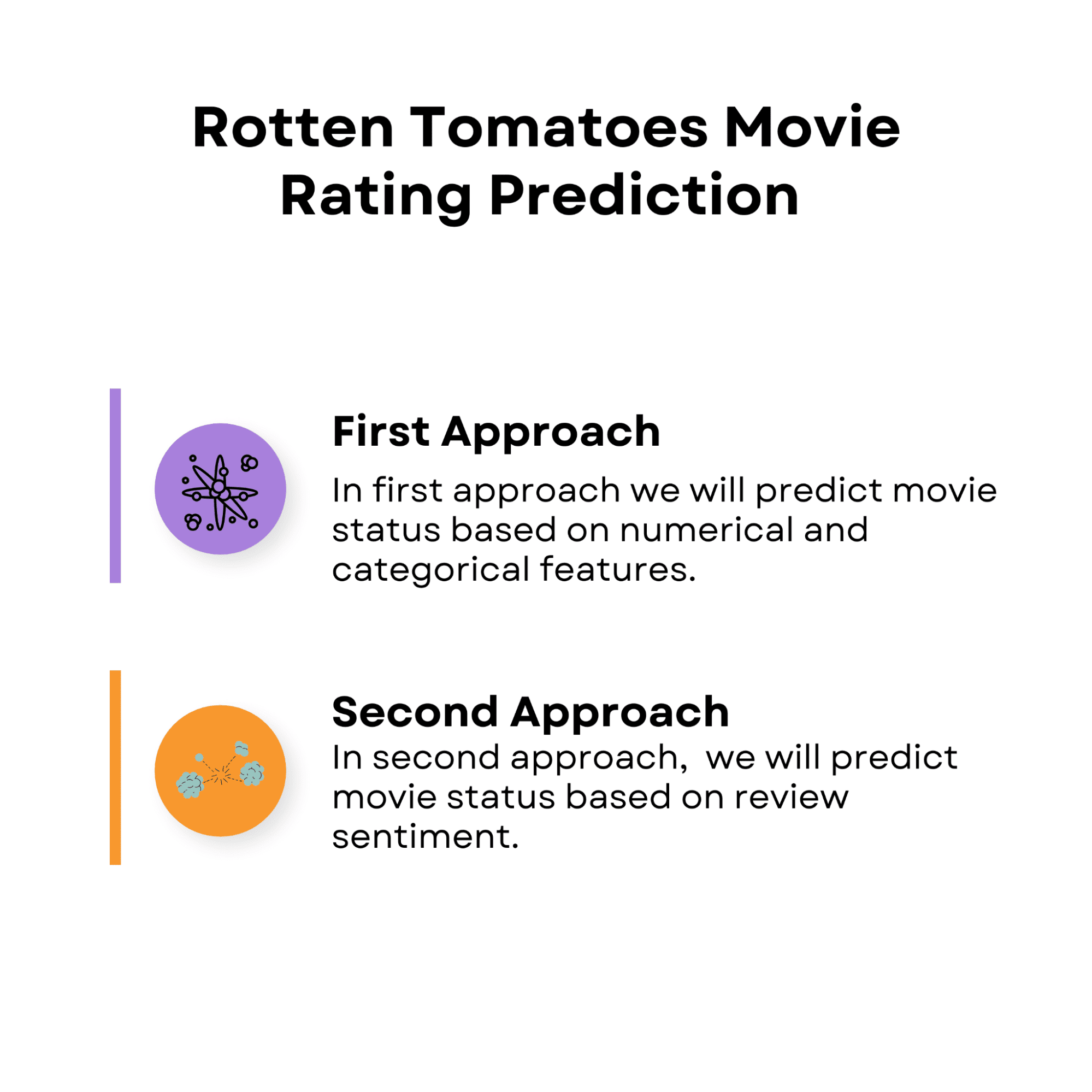
Image by Author
Throughout our exploration, we will discuss data preprocessing, various classifiers, and potential improvements to enhance the performance of our models.
By the end of this post, you will have gained an understanding of how machine learning can be employed to predict movie success and how this knowledge can be applied in the entertainment industry.
But before going deeper, let’s discover the data we will work on.
First Approach: Predicting Movie Status Based on Numerical and Categorical Features
In this approach, we will use a combination of numerical and categorical features to predict the success of a movie.
The features we will consider include factors such as budget, genre, runtime, and director, among others.
We will employ several machine learning algorithms to build our models, including Decision Trees, Random Forests, and Weighted Random Forests with feature selection.
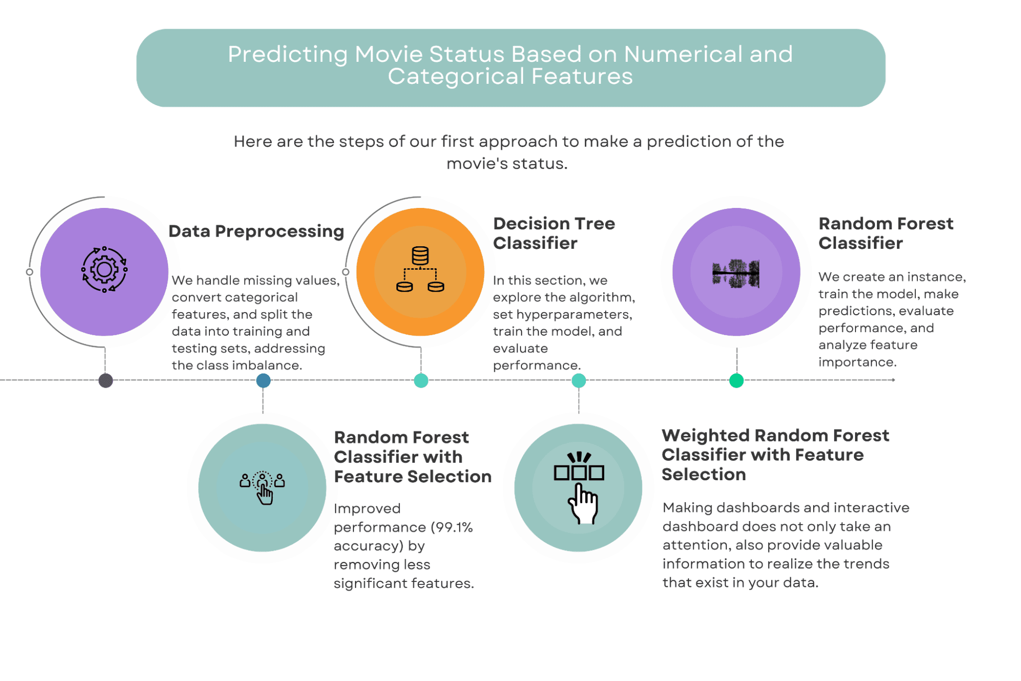
Image by Author
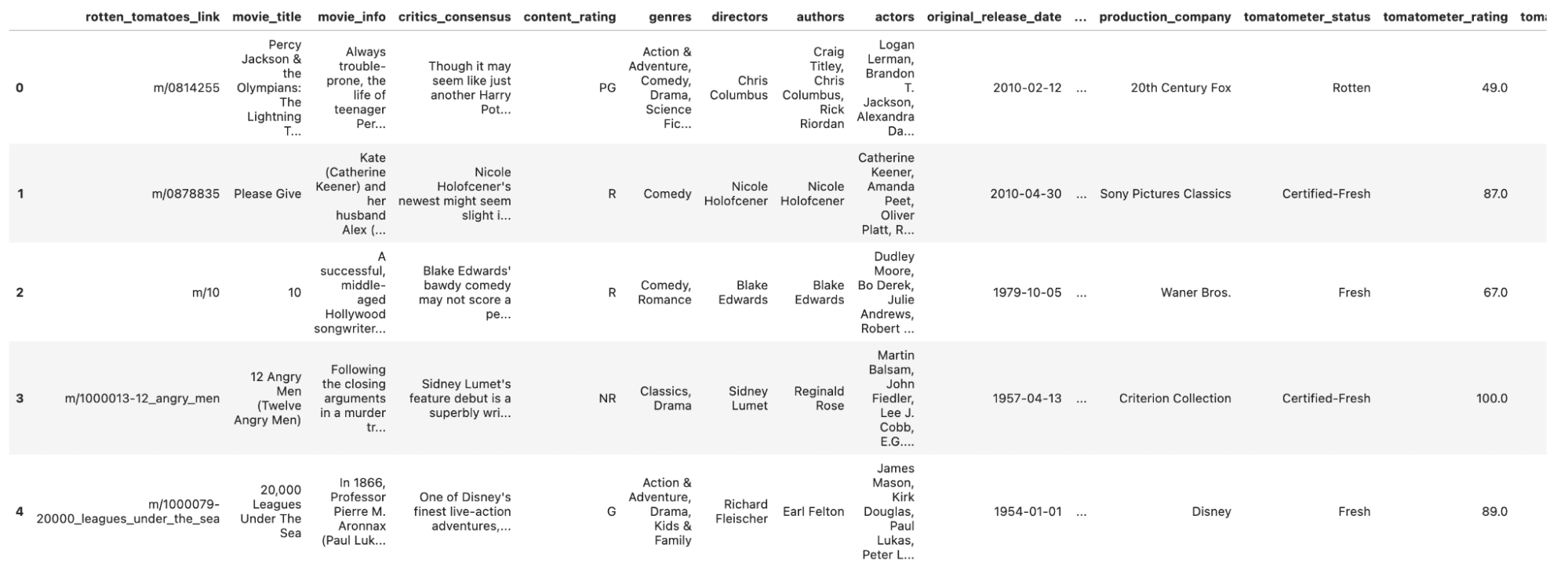
Let’s read our data and take a glimpse of it.
Here is the code.
df_movie = pd.read_csv('rotten_tomatoes_movies.csv')
df_movie.head()
Here is the output.
Now, let’s start with Data Preprocessing.
There are many columns in our Data set.
Let’s see.
To develop a better understanding of the statistical features, let’s use describe the () method. Here is the code.
df_movie.describe()
Here is the output.

Now, we have a quick overview of our data, let’s go to the preprocessing stage.
Data Preprocessing
Before we can begin building our models, it's essential to preprocess our data.
This involves cleaning the data by handling categorical features and converting them into numerical representations, and scaling the data to ensure that all features have equal importance.
We first examined the content_rating column to see the unique categories and their distribution in the dataset.
print(f'Content Rating category: {df_movie.content_rating.unique()}')
Then, we will create a bar plot to see the distribution of each content rating category.
ax = df_movie.content_rating.value_counts().plot(kind='bar', figsize=(12,9))
ax.bar_label(ax.containers[0])
Here is the full code.
print(f'Content Rating category: {df_movie.content_rating.unique()}')
ax = df_movie.content_rating.value_counts().plot(kind='bar', figsize=(12,9))
ax.bar_label(ax.containers[0])
Here is the output.
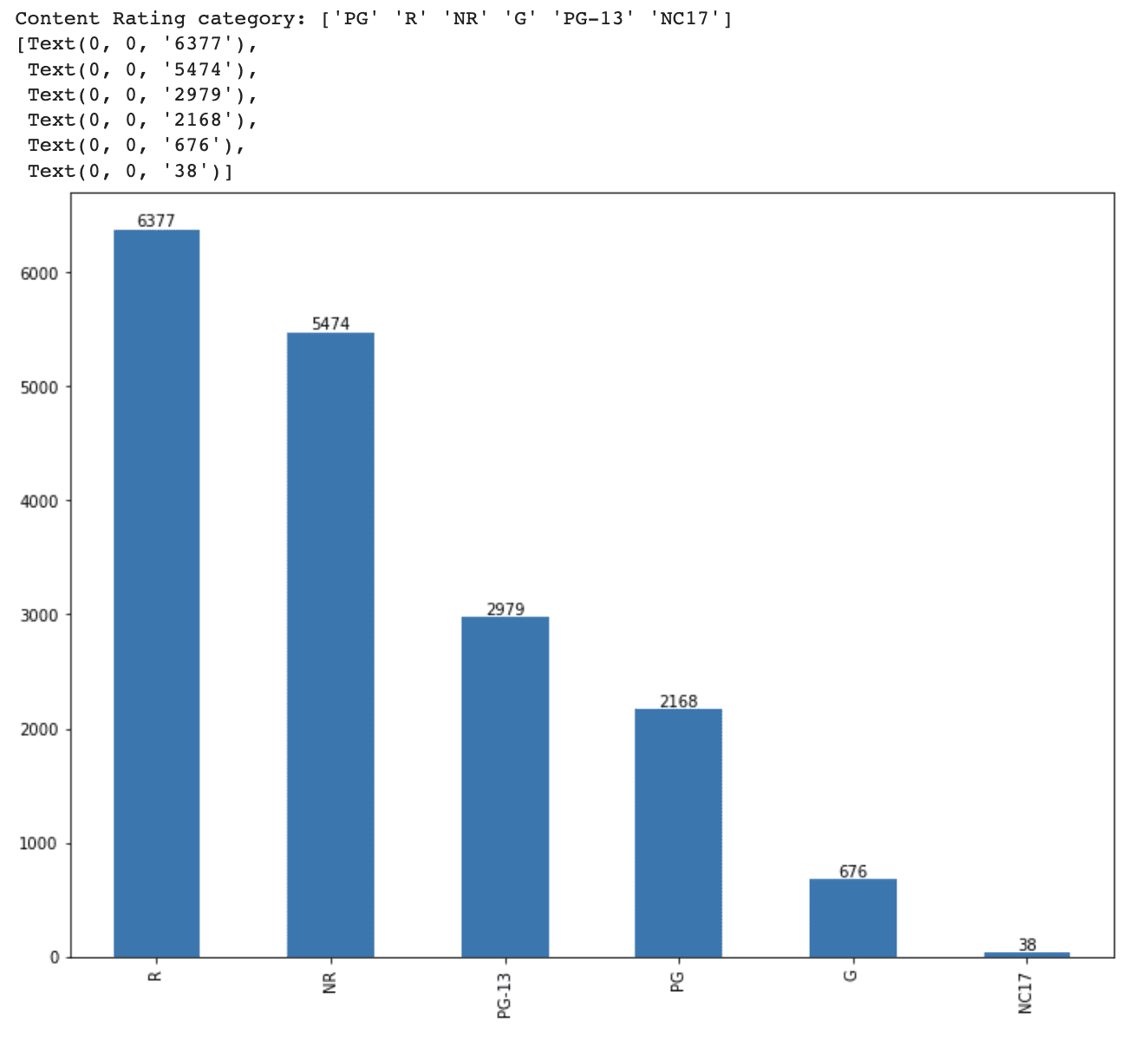
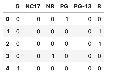
It is essential to convert categorical features into numeric forms for our machine learning models which need numeric inputs. For multiple elements in this data science project, we are going to apply two generally accepted methods: ordinal encoding and one-hot encoding. Ordinal encoding is better when categories imply a degree of intensity, but the one-hot encoding is ideal when no magnitude representation is provided. For the "content_rating" assets, we will use a one-hot encoding method.
Here is the code.
content_rating = pd.get_dummies(df_movie.content_rating)
content_rating.head()
Here is the output.
Let's go ahead and process another feature, audience_status.
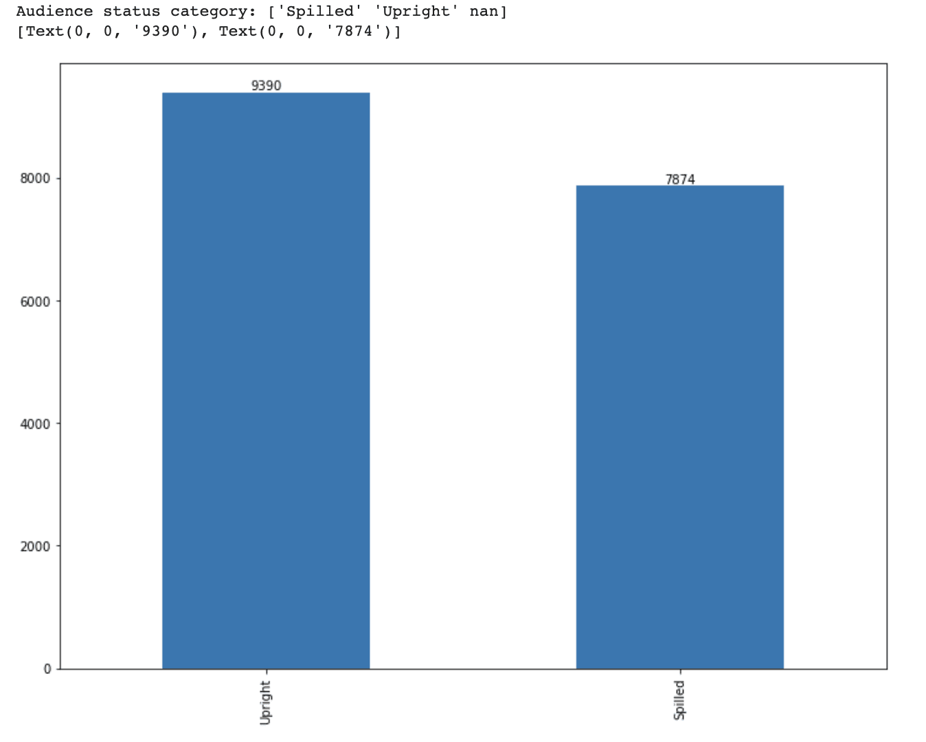
This variable has two options: 'Spilled' and 'Upright'.
We did already apply one hot coding, so now it is time to transform this categorical variable into a numerical one by using ordinal encoding.
Because each category illustrates an order of magnitude, we will transform these into numerical values by using ordinal encoding.
As we did earlier, first let’s find the unique audience status.
print(f'Audience status category: {df_movie.audience_status.unique()}')
Then, let’s create a bar plot and print out the values on top of bars.
# Visualize the distribution of each category
ax = df_movie.audience_status.value_counts().plot(kind='bar', figsize=(12,9))
ax.bar_label(ax.containers[0])
Here is the full code.
print(f'Audience status category: {df_movie.audience_status.unique()}')
# Visualize the distribution of each category
ax = df_movie.audience_status.value_counts().plot(kind='bar', figsize=(12,9))
ax.bar_label(ax.containers[0])
Here is the output.
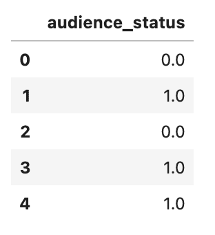
Okay, now it is time to do ordinal coding by using replace method.
Then let’s view the first five rows by using the head() method.
Here is the code.
# Encode audience status variable with ordinal encoding
audience_status = pd.DataFrame(df_movie.audience_status.replace(['Spilled','Upright'],[0,1]))
audience_status.head()
Here is the output.
Since our target variable, tomatometer_status, have three distinct categories, 'Rotten', 'Fresh', and 'Certified-Fresh', these categories also represent an order of magnitude.
That’s why we again will do ordinal encoding to transform these categorical variables into numerical variables.
Here is the code.
# Encode tomatometer status variable with ordinal encoding
tomatometer_status = pd.DataFrame(df_movie.tomatometer_status.replace(['Rotten','Fresh','Certified-Fresh'],[0,1,2]))
tomatometer_status
Here is the output.
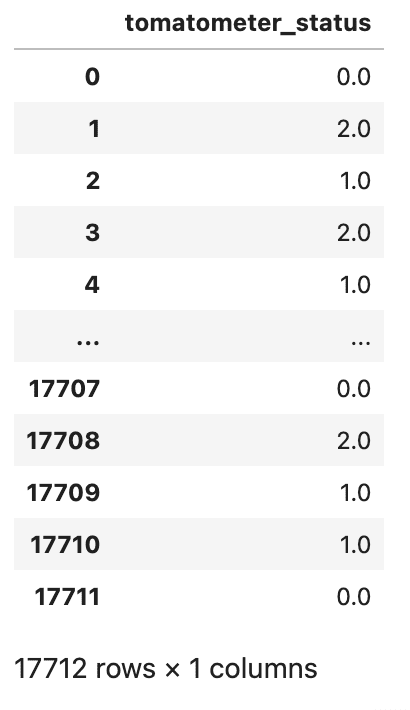
After changing categorial to numerical, it is now time to combine the two data frames. We'll use Pandas pd.concat() function for this, and the dropna() method to remove rows with missing values across all columns.
Following that, we'll use the head function to look at the freshly formed DataFrame.
Here is the code.
df_feature = pd.concat([df_movie[['runtime', 'tomatometer_rating', 'tomatometer_count', 'audience_rating', 'audience_count', 'tomatometer_top_critics_count', 'tomatometer_fresh_critics_count', 'tomatometer_rotten_critics_count']], content_rating, audience_status, tomatometer_status], axis=1).dropna()
df_feature.head()
Here is the output.

Great, now let’s inspect our numerical variables by using describe method.
Here is the code.
df_feature.describe()
Here is the output.

Now let’s check the length of our DataFrame by using len method.
Here is the code.
len(df)
Here is the output.

After removing rows with missing values and doing the transformation for building machine learning, now our data frame has 17017 rows.
Let’s now analyze the distribution of our target variables.
As we keep constantly doing since the beginning, we will draw a bar graph and put the values at the top of the bar.
Here is the code.
ax = df_feature.tomatometer_status.value_counts().plot(kind='bar', figsize=(12,9))
ax.bar_label(ax.containers[0])
Here is the output.

Our dataset contains 7375 'Rotten,' 6475 'Fresh,' and 3167 'Certified-Fresh' films, indicating a class imbalance issue.
The problem will be addressed at a later time.
For the time being, let’s split our dataset into testing and training sets using an 80% to 20% split.
Here is the code.
X_train, X_test, y_train, y_test = train_test_split(df_feature.drop(['tomatometer_status'], axis=1), df_feature.tomatometer_status, test_size= 0.2, random_state=42)
print(f'Size of training data is {len(X_train)} and the size of test data is {len(X_test)}')
Here is the output.

Decision Tree Classifier
In this section, we will look at the Decision Tree Classifier, a machine learning technique that is commonly used for classification problems and sometimes for regression.
The classifier works by dividing data points into branches, each of which has an inner node (which includes a set of conditions) and a leaf node (which has the predicted value).
Following these branches and considering the conditions (True or False), data points are separated into the proper categories. The process is seen below.
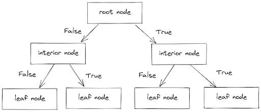
Image by Author
When we apply a Decision Tree Classifier, we can alter multiple hyperparameters, like the maximum depth of the tree and the maximum number of leaf nodes.
For our first attempt, we will limit the number of leaf nodes to three in order to make the tree simple and understandable.
To begin, we will create a Decision Tree Classifier with a maximum of three leaf nodes. This classifier will then be trained on our training data and used to generate predictions on the test data. Finally, we will examine the accuracy, precision, and recall metrics to assess the performance of our limited Decision Tree Classifier.
Now let’s implement the Decision Tree algorithm with sci-kit learn step by step.
First, let’s define a Decision Tree Classifier object with a maximum of three leaf nodes, using the DecisionTreeClassifier() function from the scikit-learn library.
The random_state parameter is used to ensure that the same results are produced each time the code is run.
tree_3_leaf = DecisionTreeClassifier(max_leaf_nodes= 3, random_state=2)
Then it is time to train the Decision Tree Classifier on the training data (X_train and y_train), using the .fit() method.
tree_3_leaf.fit(X_train, y_train)
Next, we make predictions on the test data(X_test) using the trained classifier with the predict method.
y_predict = tree_3_leaf.predict(X_test)
Here we print the accuracy score and classification report of the predicted values compared to the actual target values of the test data. We use the accuracy_score() and classification_report() functions from the scikit-learn library.
print(accuracy_score(y_test, y_predict))
print(classification_report(y_test, y_predict))
Finally, we will plot the confusion matrix to visualize the performance of the Decision Tree Classifier on the test data. We use the plot_confusion_matrix() function from the scikit-learn library.
fig, ax = plt.subplots(figsize=(12, 9))
plot_confusion_matrix(tree_3_leaf, X_test, y_test, cmap='cividis', ax=ax)
Here is the code.
# Instantiate Decision Tree Classifier with max leaf nodes = 3
tree_3_leaf = DecisionTreeClassifier(max_leaf_nodes= 3, random_state=2)
# Train the classifier on the training data
tree_3_leaf.fit(X_train, y_train)
# Predict the test data with trained tree classifier
y_predict = tree_3_leaf.predict(X_test)
# Print accuracy and classification report on test data
print(accuracy_score(y_test, y_predict))
print(classification_report(y_test, y_predict))
# Plot confusion matrix on test data
fig, ax = plt.subplots(figsize=(12, 9))
plot_confusion_matrix(tree_3_leaf, X_test, y_test, cmap ='cividis', ax=ax)
Here is the output.

It can be clearly seen from the output, our Decision Tree works well, especially taking into consideration that we limited it to three leaf nodes. One of the advantages of having a simple classifier is that the decision tree can be visualized and understandable.
Now, to understand how the decision tree makes decisions, let’s visualize the decision tree classifier by using the plot_tree method from sklearn.tree.
Here is the code.
fig, ax = plt.subplots(figsize=(12, 9))
plot_tree(tree_3_leaf, ax= ax)
plt.show()
Here is the output.
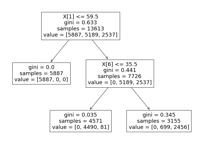
Now let’s analyze this decision tree, and find out how it carries out the decision-making process.
Specifically, the algorithm uses the 'tomatometer_rating' feature as the primary determinant of each test data point's classification.
- If the 'tomatometer_rating' is less than or equal to 59.5, the data point is assigned a label of 0 ('Rotten'). Otherwise, the classifier progresses to the next branch.
- In the second branch, the classifier uses the 'tomatometer_fresh_critics_count' feature to classify the remaining data points.
- If the value of this feature is less than or equal to 35.5, the data point is labeled as 1 ('Fresh').
- If not, it is labeled as 2 ('Certified-Fresh').
This decision-making process closely aligns with the rules and criteria that Rotten Tomatoes use to assign movie statuses.
According to the Rotten Tomatoes website, movies are classified as
- ‘Fresh' if their tomatometer_rating is 60% or higher.
- 'Rotten' if it falls below 60%.
Our Decision Tree Classifier follows a similar logic, classifying movies as 'Rotten' if their tomatometer_rating is below 59.5 and 'Fresh' otherwise.
However, when distinguishing between 'Fresh' and 'Certified-Fresh' movies, the classifier must consider several more features.
According to Rotten Tomatoes, films must meet specific criteria to be classified as 'Certified-Fresh', such as:
- Having a consistent Tomatometer score of at least 75%
- At least five reviews from top critics.
- Minimum of 80 reviews for wide-release films.
Our limited Decision Tree model only takes into account the number of reviews from top critics to differentiate between 'Fresh' and 'Certified-Fresh' movies.
Now, we understand the logic behind the Decision Tree. So to increase its performance, let’s follow the same steps but this time, we will not add the max-leaf nodes argument.
Here is the step-by-step explanation of our code. This time I won't expand the code too much as we did before.
Define the decision tree classifier.
tree = DecisionTreeClassifier(random_state=2)
Train the classifier on the training data.
tree.fit(X_train, y_train)
Predict the test data with a trained tree classifier.
y_predict = tree.predict(X_test)
Print the accuracy and classification report.
print(accuracy_score(y_test, y_predict))
print(classification_report(y_test, y_predict))
Plot confusion matrix.
fig, ax = plt.subplots(figsize=(12, 9))
plot_confusion_matrix(tree, X_test, y_test, cmap ='cividis', ax=ax)
Great now, let’s see them together.
Here's the whole code.
fig, ax = plt.subplots(figsize=(12, 9))
# Instantiate Decision Tree Classifier with default hyperparameter settings
tree = DecisionTreeClassifier(random_state=2)

# Train the classifier on the training data
tree.fit(X_train, y_train)

# Predict the test data with trained tree classifier
y_predict = tree.predict(X_test)

# Print accuracy and classification report on test data
print(accuracy_score(y_test, y_predict))
print(classification_report(y_test, y_predict))

# Plot confusion matrix on test data
fig, ax = plt.subplots(figsize=(12, 9))
plot_confusion_matrix(tree, X_test, y_test, cmap ='cividis', ax=ax)
Here is the output.
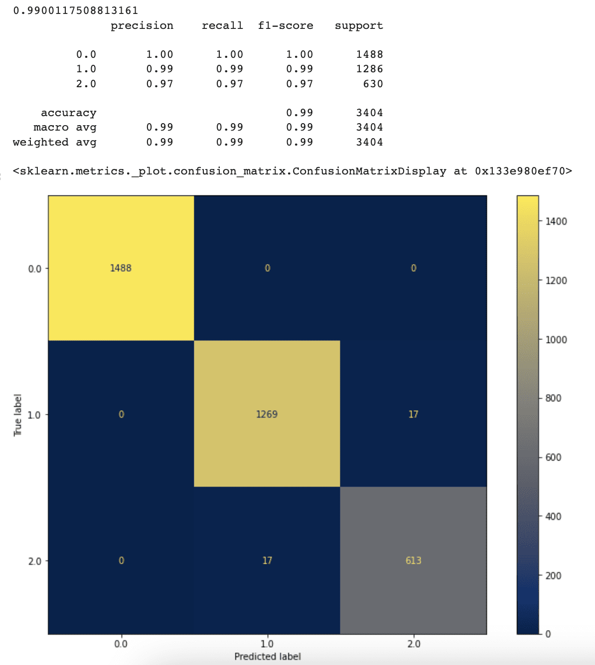
The accuracy, precision, and recall values of our classifier have increased as a result of removing the maximum leaf nodes limitation. The classifier now reaches 99% accuracy, up from 94% previously.
This displays that when we allow our classifier to pick the optimal number of leaf nodes on its own, it performs better.
Although the current result appears to be outstanding, more tuning to reach even better accuracy is still possible. In the next part, we'll look into this option.
Random Forest Classifier
Random Forest is an ensemble of Decision Tree Classifiers that have been combined into a single algorithm. It uses a bagging strategy to train each Decision Tree, which includes randomly picking training data points. Each tree is trained on a separate subset of the training data as a result of this technique.
The bagging method has become known for using a bootstrap methodology to sample data points, allowing the same data point to be picked for several Decision Trees.

Image by Author
By using scikit learn, it is really easy to apply a Random forest classifier.
Using Scikit-learn to set up the Random Forest algorithm is an easy process.
The algorithm's performance, like the performance of the Decision Tree Classifier, may be increased through changing hyperparameter values such as the number of Decision Tree Classifiers, maximum leaf nodes, and maximum tree depth.
We will use default options here first.
Let’s see the code step-by-step again.
First, let’s instantiate a Random Forest Classifier object using the RandomForestClassifier() function from the scikit-learn library, with a random_state parameter set to 2 for reproducibility.
rf = RandomForestClassifier(random_state=2)
Then, train the Random Forest Classifier on the training data (X_train and y_train), using the .fit() method.
rf.fit(X_train, y_train)
Next, use the trained classifier to make predictions on the test data (X_test), using the .predict() method.
y_predict = rf.predict(X_test)
Then, print the accuracy score and classification report of the predicted values compared to the actual target values of the test data.
We use the accuracy_score() and classification_report() functions from the scikit-learn library again.
print(accuracy_score(y_test, y_predict))
print(classification_report(y_test, y_predict))
Finally, let’s plot a confusion matrix to visualize the performance of the Random Forest Classifier on the test data. We use the plot_confusion_matrix() function from the scikit-learn library.
fig, ax = plt.subplots(figsize=(12, 9))
plot_confusion_matrix(rf, X_test, y_test, cmap ='cividis', ax=ax)
Here is the whole code.
# Instantiate Random Forest Classifier
rf = RandomForestClassifier(random_state=2)

# Train Random Forest Classifier on training data
rf.fit(X_train, y_train)

# Predict test data with trained model
y_predict = rf.predict(X_test)

# Print accuracy score and classification report
print(accuracy_score(y_test, y_predict))
print(classification_report(y_test, y_predict))

# Plot confusion matrix
fig, ax = plt.subplots(figsize=(12, 9))
plot_confusion_matrix(rf, X_test, y_test, cmap ='cividis', ax=ax)
Here is the output.

The accuracy and confusion matrix results show that the Random Forest algorithm outperforms the Decision Tree Classifier. This shows the advantage of ensemble approaches such as Random Forest over individual classification algorithms.
Furthermore, tree-based machine learning methods allow us to identify the significance of each feature once the model has been trained. For this reason, Scikit-learn provides the feature_importances_ function.
Great, once again, let’s see the code step by step to understand it.
First, the feature_importances_ attribute of the Random Forest Classifier object is used to obtain the importance score of each feature in the dataset.
The importance score indicates how much each feature contributes to the prediction performance of the model.
# Get the feature importance
feature_importance = rf.feature_importances_
Next, the feature importances are printed out in descending order of importance, along with their corresponding feature names.
# Print feature importance
for i, feature in enumerate(X_train.columns):
    print(f'{feature} = {feature_importance[i]}')
Then to visualize features from the most important to least important, let’s use argsort() method from the numpy.
# Visualize feature from the most important to the least important
indices = np.argsort(feature_importance)
Finally, a horizontal bar chart is created to visualize the feature importances, with features ranked from most to least important on the y-axis and the corresponding importance scores on the x-axis.
This chart allows us to easily identify the most important features in the dataset and to determine which features have the greatest impact on the model's performance.
plt.figure(figsize=(12,9))
plt.title('Feature Importances')
plt.barh(range(len(indices)), feature_importance[indices], color='b', align='center')
plt.yticks(range(len(indices)), [X_train.columns[i] for i in indices])
plt.xlabel('Relative Importance')
plt.show()
Here is the whole code.
# Get the fature importance
feature_importance = rf.feature_importances_

# Print feature importance
for i, feature in enumerate(X_train.columns):
    print(f'{feature} = {feature_importance[i]}')

# Visualize feature from the most important to the least important
indices = np.argsort(feature_importance)

plt.figure(figsize=(12,9))
plt.title('Feature Importances')
plt.barh(range(len(indices)), feature_importance[indices], color='b', align='center')
plt.yticks(range(len(indices)), [X_train.columns[i] for i in indices])
plt.xlabel('Relative Importance')
plt.show()
Here is the output.
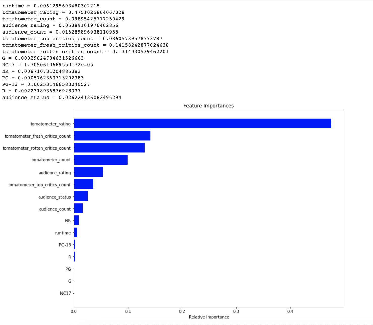
By seeing this graph, it is clear that NR, PG-13, R, and runtime did not consider important by the model for predicting unseen data points. In the next section, whether let’s see addressing this issue can increase our model's performance or not.
Random Forest Classifier with Feature Selection
Here is the code.
In the last section, we discovered that some of our features were considered less significant by our Random forest model, in making predictions.
As a result, to enhance the model’s performance, let’s exclude these less relevant features including NR, runtime, PG-13, R, PG, G, and NC17.
In the following code, we will get the feature importance first, then we will split to train and test set, but inside the code block we dropped these less significant features. Then we will print out the train and test set size.
Here is the code.
# Get the feature importance
feature_importance = rf.feature_importances_
X_train, X_test, y_train, y_test = train_test_split(df_feature.drop(['tomatometer_status', 'NR', 'runtime', 'PG-13', 'R', 'PG','G', 'NC17'], axis=1),df_feature.tomatometer_status, test_size= 0.2, random_state=42)
print(f'Size of training data is {len(X_train)} and the size of test data is {len(X_test)}')
Here is the output.

Great, since we dropped these less significant features, let’s see whether our performance increased or not.
Because we did this too many times, I quickly explain the following codes.
In the following code, we first initialize a random forest classifier and then train the random forest on the training data.
rf = RandomForestClassifier(random_state=2)

rf.fit(X_train, y_train)
Then we calculate the accuracy score and classification report by using test data and print them out.
print(accuracy_score(y_test, y_predict))
print(classification_report(y_test, y_predict))
Finally, we plot the confusion matrix.
fig, ax = plt.subplots(figsize=(12, 9))
plot_confusion_matrix(rf, X_test, y_test, cmap ='cividis', ax=ax)
Here is the whole code.
# Initialize Random Forest class
rf = RandomForestClassifier(random_state=2)

# Train Random Forest on the training data after feature selection
rf.fit(X_train, y_train)

# Predict the trained model on the test data after feature selection
y_predict = rf.predict(X_test)

# Print the accuracy score and the classification report
print(accuracy_score(y_test, y_predict))
print(classification_report(y_test, y_predict))

# Plot the confusion matrix
fig, ax = plt.subplots(figsize=(12, 9))
plot_confusion_matrix(rf, X_test, y_test, cmap ='cividis', ax=ax)
Here is the output.
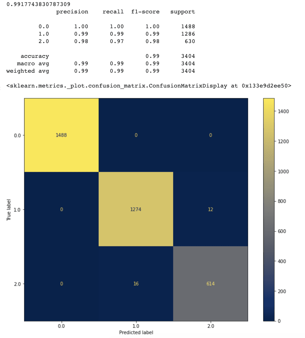
It looks like our new approach works quite well.
After doing feature selection, accuracy has increased to 99.1 %.
Our model's false positive and false negative rates have also lowered marginally when compared to the prior model.
This indicates that having more characteristics does not always imply a better model. Some insignificant characteristics may create noise which might be the reason for lowering the model's prediction accuracy.
Now since our model’s performance has increased that far, let’s discover other methods to check if we can increase more.
Weighted Random Forest Classifier with Feature Selection
In the first section, we realized that our features were a little imbalanced. We have three different values, Rotten' (represented by 0), 'Fresh' (represented by 1), and 'Certified-Fresh' (represented by 2).
First, let’s see the distribution of our features.
Here's the code for visualizing the label distribution.
ax = df_feature.tomatometer_status.value_counts().plot(kind='bar', figsize=(12,9))
ax.bar_label(ax.containers[0])
Here is the output.

It is clear that the amount of data with the ‘Certified Fresh’ feature is much less than the others.
To solve the issue of data imbalance, we can use approaches such as the SMOTE algorithm to oversample the minority class or provide class weight information to the model during the training phase.
Here we will use the second approach.
To compute class weight, we will use the compute_class_weight() function from the scikit-learn library.
Inside this function, the class_weight parameter is set to 'balanced' to account for imbalanced classes, and the classes parameter is set to the unique values in the tomatometer_status column of df_feature.
The y parameter is set to the values of the tomatometer_status column in df_feature.
class_weight = compute_class_weight(class_weight= 'balanced', classes= np.unique(df_feature.tomatometer_status),
                      y = df_feature.tomatometer_status.values)
Then, the dictionary is created to map the class weights to their respective indices.
This is done by converting the class weight list to a dictionary using the dict() function and zip() function.
The range() function is used to generate a sequence of integers corresponding to the length of the class weight list, which is then used as the keys for the dictionary.
class_weight_dict = dict(zip(range(len(class_weight.tolist())), class_weight.tolist()
Finally, let’s see our dictionary.
class_weight_dict
Here is the whole code.
class_weight = compute_class_weight(class_weight= 'balanced', classes= np.unique(df_feature.tomatometer_status),
                      y = df_feature.tomatometer_status.values)

class_weight_dict = dict(zip(range(len(class_weight.tolist())), class_weight.tolist()))
class_weight_dict
Here is the output.

Class 0 ('Rotten') has the least weight, while class 2 ('Certified-Fresh') has the highest weight.
When we apply our Random Forest classifier, we can now include this weight information as an argument.
The remaining code is the same as we did earlier many times.
Let's build a new Random Forest model with class weight data, train it on the training set, predict the test data, and display the accuracy score and confusion matrix.
Here is the code.
# Initialize Random Forest model with weight information
rf_weighted = RandomForestClassifier(random_state=2, class_weight=class_weight_dict)

# Train the model on the training data
rf_weighted.fit(X_train, y_train)

# Predict the test data with the trained model
y_predict = rf_weighted.predict(X_test)

#Print accuracy score and classification report
print(accuracy_score(y_test, y_predict))
print(classification_report(y_test, y_predict))

#Plot confusion matrix
fig, ax = plt.subplots(figsize=(12, 9))
plot_confusion_matrix(rf_weighted, X_test, y_test, cmap ='cividis', ax=ax)
Here is the output.

Our model's performance increased when we added class weights, and it now has an accuracy of 99.2%.
The number of correct predictions for the “Fresh “ label also increased by one.
Using class weights to address the data imbalance problem is a useful method since it encourages our model to pay more attention to labels with higher weights throughout the training phase.
Link to this data science project: https://platform.stratascratch.com/data-projects/rotten-tomatoes-movies-rating-prediction
Nate Rosidi is a data scientist and in product strategy. He's also an adjunct professor teaching analytics, and is the founder of StrataScratch, a platform helping data scientists prepare for their interviews with real interview questions from top companies. Connect with him on Twitter: StrataScratch or LinkedIn.
