Understanding Objective Functions in Neural Networks
This blog post is targeted towards people who have experience with machine learning, and want to get a better intuition on the different objective functions used to train neural networks.
By Lars Hulstaert, Data Science and Machine Learning trainee at Microsoft.
Introduction
The reason why I decided to write this blogpost is three-fold:
- Blog posts often explain optimisation methods such as stochastic gradient descent or variants thereof, but little time is spent explaining how objective functions are constructed for neural networks. Why are the mean squared error (MSE) and cross entropy log loss used as objective functions for resp. regression and classification? Why does adding a regularisation term make sense? The general idea is that by investigating objective functions one can learn why neural networks work the way they do or why they fail in other cases.
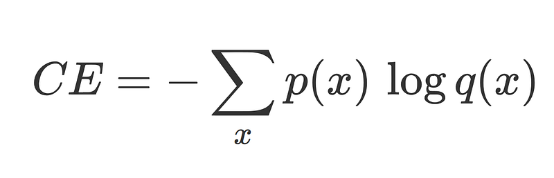
Cross entropy log loss between the ground truth p and network output q, used in classification problems.
Mean squared error between the ground truth y and network output y_tilde, used in regression problems.
- Neural networks have the reputation of providing bad probability estimates and they suffer from adversarial examples. In short: neural networks are often highly confident even when they are wrong. This can be an issue when they are deployed in real-life scenarios (e.g. self-driving cars). A self-driving car should be certain when making decisions at 90 mph. If we deploy deep learning pipelines, we should be aware of their strengths and weaknesses.
- I always wondered how neural networks can be explained from a probabilistic perspective and how they fit in the wider framework of machine learning models. People tend to talk about network outputs as probabilities. Is there a link between the probabilistic interpretation of neural networks and their objective functions?
The main inspiration for this blog post is based on the work I did on Bayesian Neural Networks with my friend Brian Trippe at the Computational and Biological Learning Lab in Cambridge University. I highly recommend anyone to read Brian's thesis on variational inference in neural networks.
Disclaimer: At the Computational and Biological Learning Lab Bayesian machine learning techniques are unapologetically taught as the way forward. As such, be aware of potential bias in this blog post. ;)
Supervised machine learning
In supervised machine learning problems, we often consider a dataset D of observation pairs (x, y) and we try to model the following distribution:
For example in image classification, x represents an image and y the corresponding image label. p(y|x, θ) represents the probability of the label y given the image x and a model defined by parameters θ.
Models that follow this approach are called discriminative models. In discriminative or conditional models the parameters that define the conditional probability distribution function p(y|x, θ) are inferred from the training data.
Based on the observed data x (input data or feature values) the model outputs a probability distribution, which is then used to predict y (class or real value). Different machine learning models require different parameters to be estimated. Both linear models (e.g. logistic regression, defined by a set of weights equal to the number of features) and non-linear models (e.g. neural networks, defined by a set of weights for each layer) can be used to approximate the conditional probability distributions.
For typical classification problems the set of learnable parameters θ is used to define a mapping from x to a categorical distribution over the different labels. A discriminative classification model produces N probabilities as output, with N equal to the number of classes. Each x belongs to a single class, but model uncertainty is reflected by outputting a distribution over the classes. Typically, the class with maximum probability is chosen when making a decision.
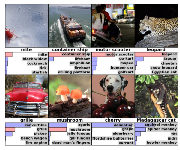
In image classification, the network outputs a categorical distribution over image classes. The image above depicts the top 5 classes (classes with highest probability) for a test image.
Note that discriminative regression models often only output a single predicted value, instead of a distribution over all the real values. This is different from discriminative classification models where a distribution over all the possible classes is provided. Does this mean discriminative models fall apart for regression? Shouldn't the output of the model tell us which regression values are more likely than others?
Although the single output of a discriminative regression model is misleading, the output of a regression model actually relates to a well-known probability distribution, the Gaussian distribution. As it turns out, the output of a discriminative regression model represents the mean of a Gaussian distribution (a Gaussian distribution is fully defined by a mean and a standard deviation). With this information, you can determine the likelihood of each real value given the input x.
Only the mean value of this distribution is typically modelled, and the standard deviation of the Gaussian is either not modelled or chosen to be constant across all x. In discriminative regression models, θ thus defines a mapping from x to the mean of a Gaussian from which y is sampled. The mean value is almost always chosen when making a decision. Models that output a mean and a standard deviation for a given x are more informative, as the model is able to express for which x it is uncertain (by increasing the standard deviation).
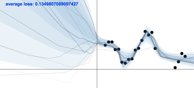
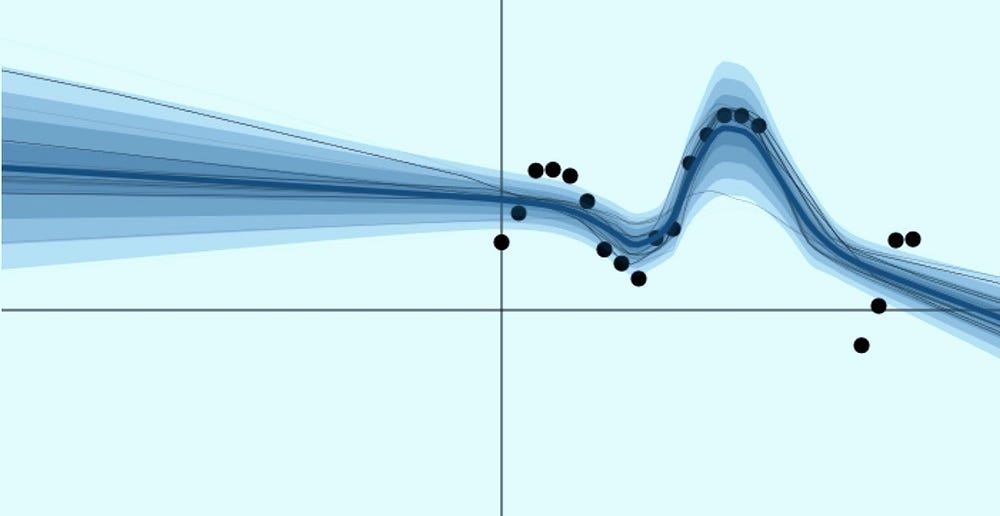
A model needs to be uncertain in regions where there is no training data and certain in regions where it has training data. Such a model is displayed in the image above, from Yarin Gal's blog post.
Other probabilistic models (such as Gaussian processes) do a significantly better job at modelling uncertainty in regression problems, whereas discriminative regression models tend to be overconfident when modelling mean and standard deviation at the same time.
A Gaussian process is able to quantify uncertainty through explicitely modelling the standard deviation. The only downside of Gaussian processes is that they do not scale well to large datasets. In the image below you can see that the GP model has small confidence intervals (determined with the standard deviation) around regions with a lot of data. In regions with few data points, the confidence intervals become significantly larger.
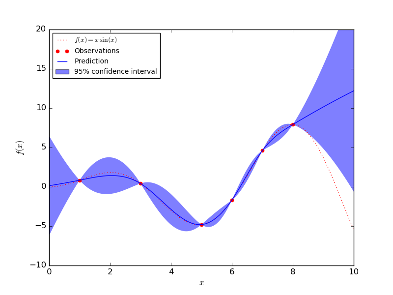
A Gaussian Process model is certain at the data points, but uncertain at other places (image taken from Sklearn)
A discriminative model is trained on the training dataset in order to learn the properties in the data that represent a class or real value. A model performs well if it is able to assign high probability to the correct class of samples or a mean that is close to the true value in the test dataset.
Link with neural networks
When neural networks are trained for a classification or regression task, the parameters of the aforementioned distributions (categorical and Gaussian) are modelled using a neural network.
This becomes clear when we attempt to determine the maximum likelihood estimate (MLE) for the parameters θ of the neural network. The MLE corresponds with finding the parameters θ for which the likelihood (or equivalent log likelihood) of the train data is maximised. More specifically, the following expression is maximised:
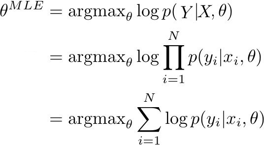
p(Y | X, θ) represents the probabilty of the true labels in the train data, when determined with the model. If p(Y | X, θ) is closer to 1, it means that the model is able to determine the correct labels/means in the train set. Given that the train data (X, Y) consists of N observation pairs, the likelihood of the train data can be rewritten as a sum of log probabilities.
In case of classification and regression, p(y|x, θ), the posterior probability for a single pair (x, y), can be rewritten as the categorical and the Gaussian distribution. In case of optimising neural networks, the goal is to shift the parameters in such a way that for a set of inputs X, the correct parameters of the probability distribution Y are given at the output (the regression value or class). This is typically achieved through gradient descent or variants thereof. In order to obtain a MLE estimate, the goal is to thus to optimise the model output with respect to the true output:
- Maximising the log of a categorical distribution corresponds with minimising the cross entropy between the approximated distribution and the true distribution.
- Maximising the log of a Gaussian distribution corresponds with minimising the mean squared error between the approximated mean and true mean.
The expression in the previous image can thus be rewritten, and results in respectively the cross entropy loss and the mean squared error, the objective functions for neural networks for classification regression.
The non-linear function that a neural network learns to go from input to probabilities or means is hard to interpret compared to more traditional probabilistic models. While this is a significant downside of neural networks, the breadth of complex functions that a neural network is able to model also brings significant advantages. Based on the derivation in this section it is clear that the objective functions for neural networks that arise when determining the MLE of the parameters can be interpreted probabilistically.
An interesting interpretation of neural networks is their relation to generalised linear models (linear regression, logistic regression, ...). Instead of taking a linear combination of the features (as one does in GLM's), a neural network produces a highly non-linear combination of features.
Maximum-a-posteriori
But, if neural networks can be interpreted as probabilistical models, why do they provide bad probability estimates and suffer from adversarial examples? Why do they require so much data?
I like to think of different models (logistic regression, neural networks, ...) as looking for good function approximators in different search spaces. While having an extremely large search space means that you have a lot of flexibility when modelling the posterior probability, it also comes at a cost. Neural networks for example are proven to be universal function approximators. This means that with enough parameters they can approximate any function (awesome!). However, in order to ensure the function is well calibrated across the entire data space, exponentially large data sets are required (expensive!).
It is important to know that a standard neural network is typically optimised using MLE. Optimisation using MLE tends to overfit to the train data and a lot of data is required to obtain decent results. The goal in machine learning is not to find a model that explains the training data well. You rather try to find a model that generalises well to unseen data, and is unsure for data that is significantly different from the train data.
Using a maximum-a-posteriori (MAP) approach is a valid alternative that is often explored when a probabilistic model suffers from overfitting. So what does MAP correspond to in the context of neural networks? What impact does it have on the objective function?
Similar to MLE, MAP can also be rewritten as an objective function in the context of neural networks. Essentially, with MAP, you are maximising the probability of a set of parameters θ given the data while assuming a prior distribution on θ:
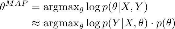
With MLE, only the first element of the formula is taken into account (how well the model explains the train data). With MAP, it is also important that the model satisfies prior assumptions (how well does θ fit the priors) in order to reduce overfitting.
Putting a Gaussian prior with 0 mean on θ corresponds with L2 regularisation added to the objective (ensuring a lot of small weights), whereas putting a Laplacian prior on θ corresponds with L1 regularisation added to the objective (ensuring a lot of weights with value 0).
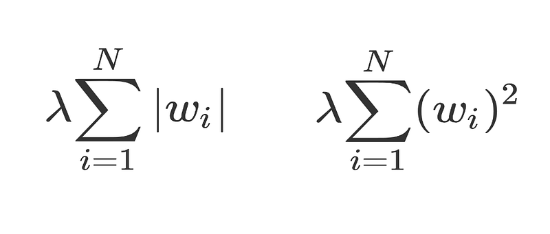
L1 regularisation on the left and L2 regularisation on the right.
A full Bayesian approach
Both in the case of MLE and MAP a single model (with a single set of parameters) is used. Especially for complex data, such as images, it is not unlikely that certain regions in the data space are not well covered. The output of the model in these regions depends on the random initialisation of the model and the training procedure, resulting in poor probability estimates for points in uncovered segments of the data space.
Although MAP ensures that the model does not overfit too much in these regions, it still results in models that are too confident. In a full Bayesian approach, this is resolved by averaging out over multiple models, resulting in better uncertainty estimates. Instead of a single set of parameters, the goal is to model a distribution over the parameters. If all models (different parameter settings) provide different estimates in uncovered regions, this indicates large uncertainty in that region. By averaging out over these models, the end result is a model that is uncertain in those regions. This is exactly what we want!
In the next blog post I will discuss Bayesian Neural Networks and how they attempt to solve the aforementioned problems of traditional neural networks. Bayesian Neural Networks (BNN’s) are still a work of active research, and there is no clear winner approach when training them.
I highly recommend the blog post by Yarin Gal on Uncertainty in Deep Learning!
Bio: Lars Hulstaert is a Data Science and Machine Learning trainee at Microsoft. Previously, he did a Masters at Cambridge University, after finishing his Engineering studies at Ghent University.
Original. Reposted with permission.
Related: