Interpretable Neural Networks with PyTorch
Learn how to build feedforward neural networks that are interpretable by design using PyTorch.

Photo by Jan Schulz # Webdesigner Stuttgart on Unsplash
There are several approaches to rate machine learning models, two of them being accuracy and interpretability. A model with high accuracy is what we usually call a good model, it learned the relationship between the inputs X and outputs y well.
If a model has high interpretability or explainability, we understand how the model makes a prediction and how we can influence this prediction by changing input features. While it is hard to say how the output of a deep neural network behaves when we increase or decrease a certain feature of the input, for a linear model it is extremely easy: if you increase the feature by one, the output increases by the coefficient of that feature. Easy.
Now, you have probably often heard something like this:
“There are interpretable models an there are well-performing models.” — someone who doesn’t know it better
However, if you have read my article about the Explainable Boosting Machine (EBM), then you already know that this is not true. The EBM is an example of a model that has a great performance while being interpretable.
The Explainable Boosting Machine
For my old article, I created the following figure displaying how we can place some models in the interpretability-accuracy space.
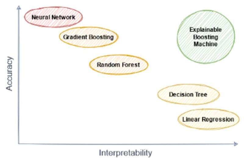
Image by the author.
In particular, I placed the deep neural networks (omitting the deep) more in the very accurate, but hard to explain region. Sure, you can mitigate the interpretability issue to some extent by using libraries like shap or lime, but these approaches come with their own set of assumptions and problems. So, let us take another path and create a neural network architecture that is interpretable by design in this article.
Disclaimer: The architecture that I am about to present just came to my mind. I do not know if there is literature about it already, at least I could not find anything. But if you know of any paper that does what I am doing here, please let me know! I will put it in the references then.
Interpretable Architecture Idea
Please note that I expect that you know how feedforward neural networks work. I will not give a full introduction here because there are many great resources about it already.
Consider the following toy neural network, having three input nodes x₁, x₂, x₃, a single output node ŷ, and three hidden layers with six nodes each. I omitted bias terms here.
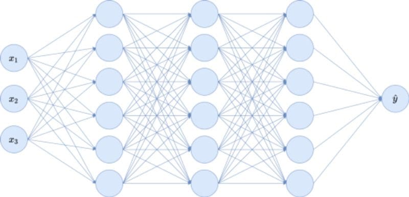
Image by the author.
The problem with this architecture for interpretability is that the inputs get all completely mixed together because of the fully connected layers. Each single input node influences all hidden layer nodes, and this influence gets more complicated the deeper we go into the network.
Inspiration by Trees
It is usually the same for tree-based models because a decision tree can potentially use every feature to create a split if we do not restrict it. For example, standard gradient boosting and its derivations like XGBoost, LightGBM, and CatBoost are not really interpretable on their own.
However, you can make gradient boosting interpretable by using decision trees that only depend on a single feature, as done with the EBM (read my article about it! ????).
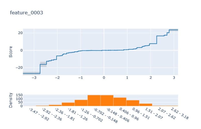
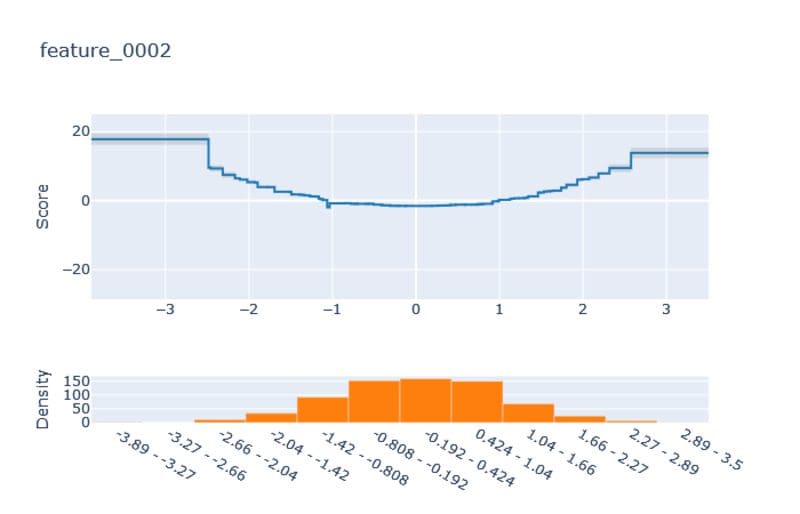
Restricting the trees like this does not hurt the performance too much in many cases, but enables us to visualize the feature impacts like this:
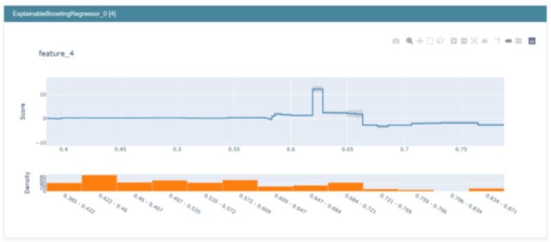
The output of interpretml’s show function. Image by the author.
Just take a look at the top part of the graphic with the blue line. It shows the impact of feature_4 on the output in some regression problem. On the x-axis, you can see the range of feature_4. The y-axis shows the Score, which is the value by how much the output is changed. The histogram below shows you the distribution of feature_4.
We can see the following from the graphic:
- If feature_4 is about 0.62, the output increases by about 10 compared to feature_4 being 0.6 or 0.65.
- If feature_4 is larger than 0.66, the impact on the output is negative.
- Changing feature_4 in the range 0.4 to 0.56 a bit does change the output much.
The final prediction of the model is then just the sum of the different feature scores. This behavior is similar to Shapley values but without the need to compute them. Great, right? Now, let me show you how we can do the same for neural networks.
Remove Edges
So, if the problem is that the inputs of the neural network get scattered all around the hidden layers because of too many edges, let us just remove some. In particular, we have to remove edges that allow information of one feature to flow to another feature. Deleting only these spilling edges, the toy neural network from above becomes:
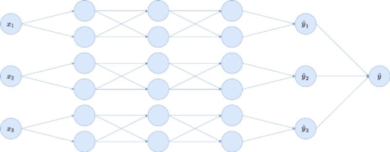
Image by the author.
We created three separate blocks for the three input variables, each block being a fully connected network with a single partial output ŷᵢ . As the last step, these ŷᵢ are summed, and a bias (omitted in the graphic) is added to produce the final output ŷ.
We introduced the partial outputs to be able to create the same kind of plots that the EBM allows. One single block in the picture above allows for one plot: xᵢ goes in, ŷᵢ comes out. We will see how to do this later.
Here we already have the complete architecture! I think it is quite easy to understand it in theory, but let us also implement it. In this way, you are happy because you can employ neural networks, and the business is happy because the neural networks are interpretable.
Implementation in PyTorch
I do not expect that you are completely familiar with PyTorch, so I will explain some basics on the way that will help you understand our custom implementation. If you know the PyTorch basics, you can skip the Fully Connected Layers section. If you have not installed PyTorch, choose your version here.
Fully Connected Layers
These layers are also known as linear in PyTorch or dense in Keras. They connect n input nodes to m output nodes using nm edges with multiplication weights. This is basically a matrix multiplication plus an addition of a bias term, as you can see in the following two code snippets:
import torchtorch.manual_seed(0) # keep things reproduciblex = torch.tensor([1., 2.]) # create an input array
linear_layer = torch.nn.Linear(2, 3) # define a linear layer
print(linear_layer(x)) # putting the input array into the layer# Output:
# tensor([ 0.7393, -1.0621,  0.0441], grad_fn=<AddBackward0>)
This is how you can create fully connected layers and apply them to PyTorch tensors. You can get the matrix that is used for the multiplication via linear_layer.weight and the bias via linear_layer.bias . Then you can do
print(linear_layer.weight @ x + linear_layer.bias) # @ = matrix mult# Output:
# tensor([ 0.7393, -1.0621,  0.0441], grad_fn=<AddBackward0>)
Nice, it’s the same! Now, the great part about PyTorch, Keras, and co. is that you can stack many of these layers together to create a neural network. In PyTorch, you can achieve this stacking via torch.nn.Sequential . To recreate the dense network from above, you could do a simple
model = torch.nn.Sequential(
    torch.nn.Linear(3, 6),
    torch.nn.ReLU(),
    torch.nn.Linear(6, 6),
    torch.nn.ReLU(),
    torch.nn.Linear(6, 6),
    torch.nn.ReLU(),
    torch.nn.Linear(6, 1),
)print(model(torch.randn(4, 3))) # feed it 4 random 3-dim. vectors
Note: I have not shown you how to train this network so far, it is just the definition of the architecture, including the initialization of the parameters. But you can feed the network three dimensional inputs and receive one dimensional outputs.
Since we want to create our own layer, let us practice with something easy first: recreating PyTorch’s Linear layer. Here is how you can do it:
import torch
import mathclass MyLinearLayer(torch.nn.Module):
    def __init__(self, in_features, out_features):
        super().__init__()
        self.in_features = in_features
        self.out_features = out_features

        # multiplicative weights
        weights = torch.Tensor(out_features, in_features)
        self.weights = torch.nn.Parameter(weights)
        torch.nn.init.kaiming_uniform_(self.weights)

        # bias
        bias = torch.Tensor(out_features)
        self.bias = torch.nn.Parameter(bias)
        bound = 1 / math.sqrt(in_features)
        torch.nn.init.uniform_(self.bias, -bound, bound)    def forward(self, x):
        return x @ self.weights.t() + self.bias
This code deserved some explanation. In the first bold block, we introduce the weights of the linear layer by
- creating a PyTorch tensor (containing all zeroes, but this does not matter)
- registering it as a learnable parameter to the layer meaning that gradient descent can update it during the training, and then
- initializing the parameters.
Initializing parameters of a neural network is a whole topic on its own, so we will not go down the rabbit hole. If it bothers you too much, you can also initialize it differently, for example via using a standard normal distribution torch.randn(out_features, in_features) , but chances are that training is slower then. Anyway, we do the same for the bias.
Then, the layer needs to know the mathematical operations it should perform in the forward method. This is just the linear operation, i.e. a matrix multiplication and addition of the bias.
Okay, now we are ready to implement the layer for our interpretable neural network!
Block Linear Layers
We now design a BlockLinear layer that we will use in the following way: First, we start with n features. The BlockLinear layer should then create n blocks consisting of h hidden neurons. To simplify things, h is the same in each block, but you can generalize this of course. In total, the first hidden layer will consist of nh neurons, but also only nh edges are connected to them (instead of n²h for a fully connected layer). To understand it better, see the picture from above again. here, n = 3, h = 2.

Image by the author.
Then — after using some non-linearity like ReLU — we will put another BlockLinear layer behind this one because the different blocks should not be merged again. We repeat this a lot until we use a Linear layer at the end to tie everything up again.
Implementation of the Block Linear Layer
Let us get to the code. It is quite similar to our custom-made linear layer, so the code should not be too intimidating.
class BlockLinear(torch.nn.Module):
    def __init__(self, n_blocks, in_features, out_features):
        super().__init__()
        self.n_blocks = n_blocks
        self.in_features = in_features
        self.out_features = out_features
        self.block_weights = []
        self.block_biases = []        for i in range(n_blocks):
            block_weight = torch.Tensor(out_features, in_features)
            block_weight = torch.nn.Parameter(block_weight)
            torch.nn.init.kaiming_uniform_(block_weight)
            self.register_parameter(
                f'block_weight_{i}',
                block_weight
            )
            self.block_weights.append(block_weight)            block_bias = torch.Tensor(out_features)
            block_bias = torch.nn.Parameter(block_bias)
            bound = 1 / math.sqrt(in_features)
            torch.nn.init.uniform_(block_bias, -bound, bound)
            self.register_parameter(
                f'block_bias_{i}',
                block_bias
            )
            self.block_biases.append(block_bias)    def forward(self, x):
        block_size = x.size(1) // self.n_blocks
        x_blocks = torch.split(
            x,
            split_size_or_sections=block_size,
            dim=1
        )        block_outputs = []
        for block_id in range(self.n_blocks):
            block_outputs.append(
                x_blocks[block_id] @ self.block_weights[block_id].t() + self.block_biases[block_id]
            )        return torch.cat(block_outputs, dim=1)
I highlighted a few lines again. The first bold lines are similar to what we have seen in our homemade linear layer, just repeated n_blocks times. This creates an independent linear layer for each block.
In the forward method, we get an x as a single tensor that we have to split into blocks again first using torch.split. As an example, a block size of 2 does the following: [1, 2, 3, 4, 5, 6] -> [1, 2], [3, 4], [5, 6]. We then apply the independent linear transformations to the different blocks, and glue the results together using torch.cat. Done!
Training the Interpretable Neural Network
Now, we have all the ingredients to define our interpretable neural network. We just have to create a dataset first:
X = torch.randn(1000, 3)
y = 3*X[:, 0] + 2*X[:, 1]**2 + X[:, 2]**3 + torch.randn(1000)
y = y.reshape(-1, 1)
We can see that we deal with a three-dimensional dataset consisting of a thousand samples here. The true relationship is linear if you square feature 1 and cube feature 2 — and this is what we want to recover with our model! So, let us define a small model that should be able to capture this relationship.
class Model(torch.nn.Module):
    def __init__(self):
        super().__init__()

        self.features = torch.nn.Sequential(
            BlockLinear(3, 1, 20),
            torch.nn.ReLU(),
            BlockLinear(3, 20, 20),
            torch.nn.ReLU(),
            BlockLinear(3, 20, 20),
            torch.nn.ReLU(),
            BlockLinear(3, 20, 1),
        )

        self.lr = torch.nn.Linear(3, 1)

    def forward(self, x):
        x_pre = self.features(x)
        return self.lr(x_pre)

model = Model()
I split the model into two steps:
- Computing the partial outputs ŷᵢ with
self.featuresand then - Compute the final prediction ŷ as a weighted sum of the ŷᵢ with
self.lr.
This makes it easier to extract the feature explanations. In the definition of self.features you can see that we create a neural network with three blocks because we have three features in the dataset. For each block, we create many hidden layers with 20 neurons per block.
Now, we can create a simple training loop:
optimizer = torch.optim.Adam(model.parameters())
criterion = torch.nn.MSELoss()for i in range(2000):
    optimizer.zero_grad()
    y_pred = model(X)
    loss = criterion(y, y_pred)
    loss.backward()
    optimizer.step()
    if i % 100 == 0:
        print(loss)
Basically, we choose Adam as an optimizer, the MSE as the loss, and then do standard gradient descent, i.e. erase old gradient with optimzer.zero_grad() , compute the predictions, compute the loss, differentiate the loss via loss.backward() and update the model parameters via optimizer.step() . You can see the training loss decline over time. We do not care about validation or test sets here. The training r² should be larger than 0.95 at the end.
We can now print the model explanations via
import matplotlib.pyplot as pltx = torch.linspace(-5, 5, 100).reshape(-1, 1)
x = torch.hstack(3*[x])for i in range(3):
    plt.plot(
        x[:, 0].detach().numpy(),
        model.get_submodule('lr').weight[0][i].item() * model.get_submodule('features')(x)[:, i].detach().numpy())
    plt.title(f'Feature {i+1}')
    plt.show()
and get
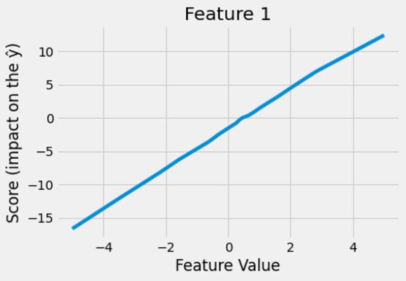
Images by the author.
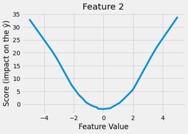
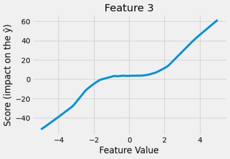
This looks pretty neat! The model figures out that the impact of feature 1 is linear, the impact of feature 2 is quadratic and the impact of feature 3 is cubic. And not only that, the model is able to show it to us, which is the great thing about the whole construction!
You can even throw the network away and make predictions solely based on these charts!
As an example, let us estimate the output of the network for x = (2, -2, 0).
- x₁ = 2 translates into a +5 for the prediction, based on the first figure.
- x₂ = -2 translates to a +9 for the prediction, based on the second figure.
- x₃ = 0 translates to a +0 for the prediction, based on the third figure.
- There is still a bias from the last linear layer that you can access via
model.get_submodule('lr').biasthis has to be added as well, but it should be small.
In total, your prediction should be around ŷ ≈ 5 + 9 + 0 + bias ≈ 14, which is fairly accurate.
You can also see what you have to do to minimize the output: choose small values for feature 1, values close to zero for feature 2, and small values for feature 3. This is something that you usually cannot see just looking at the neural network, but with the score functions, we can. That is one huge benefit of interpretability.
Note that the learned score functions from above can only be confident for regions where we actually had training data. In our dataset, we actually only observed values between -3 and 3 for each feature. Therefore, we can see that we did not get perfect x² and x³ polynomials on the edges. But I think it is still impressive that the directions of the graphs are about right. To fully appreciate this, compare it to the results of the EBM:
Images by the author.
The curves are blocky, and the extrapolation is just a straight line to both sides, which is one of the main disadvantages of tree-based methods.
Conclusion
In this article, we have talked about the interpretability of models, and how neural networks and gradient boosting fail to deliver it. While the authors of the interpretml package created the EBM, an interpretable gradient boosting algorithm, I presented to you a method to create interpretable neural networks.
We have then implemented it in PyTorch, which was a bit code-heavy, but nothing too crazy. As for the EBM, we could extract the learned score functions per feature that we can even use to make predictions.
The actual trained model is not even necessary anymore, which makes it possible to deploy and use it on weak hardware. This is because we only have to store one lookup table per feature, which is light on memory. Using a grid size of g per lookup table results in storing only O(n_features * g) elements instead of potentially millions or even billions of model parameters. Making predictions is cheap as well: just add some numbers from the lookup tables. Since this has a time complexity of only O(n_features) lookups and additions, it is much faster than a forward pass through the network.
Disclaimer again: I am not sure if this is a novel idea, but here it is anyway! If you know of any paper that explained the same idea, please leave me a message and I will reference it.
I hope that you learned something new, interesting, and useful today. Thanks for reading!
As the last point, if you
- want to support me in writing more about machine learning and
- plan to get a Medium subscription anyway,
why not do it via this link? This would help me a lot! ????
To be transparent, the price for you does not change, but about half of the subscription fees go directly to me.
Thanks a lot, if you consider supporting me!
If you have any questions, write me on LinkedIn!
Dr. Robert Kübler is a Data Scientist at Publicis Media and Author at Towards Data Science.
Original. Reposted with permission.