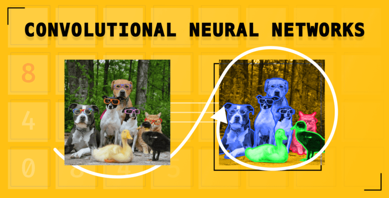
Image Classification with Convolutional Neural Networks (CNNs)
In this article, we’ll look at what Convolutional Neural Networks are and how they work.
What Is A Convolutional Neural Network (CNN)?
A Convolutional Neural Network is a special class of neural networks that are built with the ability to extract unique features from image data. For instance, they are used in face detection and recognition because they can identify complex features in image data.
How Do Convolutional Neural Networks Work?
Like other types of neural networks, CNNs consume numerical data.
Therefore, the images fed to these networks must be converted to a numerical representation. Since images are made up of pixels, they are converted into a numerical form that is passed to the CNN.
However, as we will discuss in the upcoming section, the entire numerical representation is not passed into the network. To understand how this works, let’s look at some of the steps involved in training a CNN.
Convolution
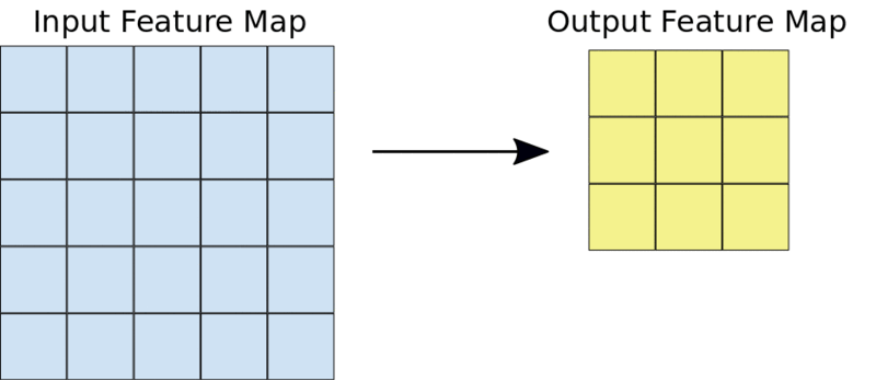
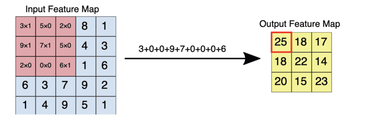
Reducing the size of the numerical representation sent to the CNN is done via the convolution operation. This process is vital so that only features that are important in classifying an image are sent to the neural network. Apart from improving the accuracy of the network, this also ensures that minimal compute resources are used in training the network.
The result of the convolution operation is referred to as a feature map, convolved feature, or activation map. Applying a feature detector is what leads to a feature map. The feature detector is also known by other names such as kernel or filter.
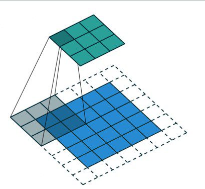
The kernel is usually a 3 by 3 matrix. Performing an element-wise multiplication of the kernel with the input image and summing the values, outputs the feature map. This is done by sliding the kernel on the input image. The sliding happens in steps known as strides. The strides and the size of the kernel can be set manually when creating the CNN.
A 3 by 3 convolutions operation.
For example, given a 5 by 5 input, a kernel of 3 by 3 will output a 3 by 3 output feature map.
Padding
In the above operations, we have seen that the size of the feature map reduces as part of applying the convolution operation. What if you want the size of the feature map to be the same size as that of the input image? That is achieved through padding.
Padding involves increasing the size of the input image by “padding” the images with zeros. As a result, applying the filter to the image leads to a feature map of the same size as the input image.
The uncolored area represents the padded area.
Padding reduces the amount of information lost in the convolution operation. It also ensures that the edges of the images are factored more often in the convolution operation.
When building the CNN, you will have the option to define the type of padding you want or no padding at all. The common options here are valid or same. Valid means no padding will be applied while same means that padding will be applied so that the size of the feature map is the same as the size of the input image.
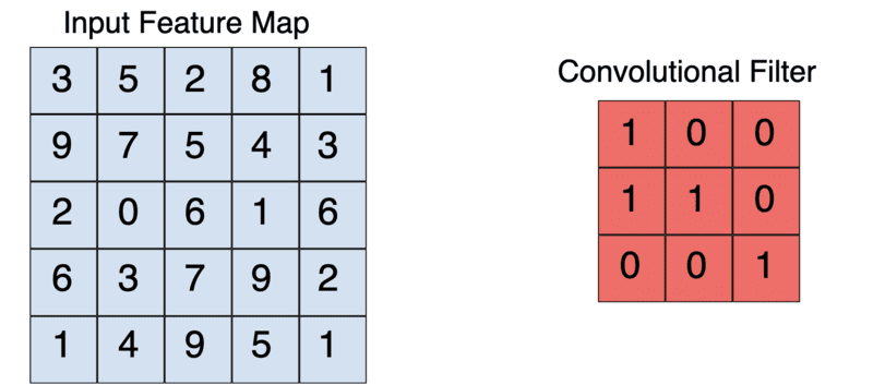
A 3 by3 kernel reduces a 5 by 5 input to a 3 by 3 output
Here is what the element-wise multiplication of the above feature map and filter would look like.
Element-wise multiplication of a 5 by input with a 3 by 3 filter.
Activation functions
A Rectified Linear Unit (ReLU) transformation is applied after every convolution operation to ensure non-linearity. ReLU is the most popular activation function but there are other activation functions to choose from.
After the transformation, all values below zero are returned as zero while the other values are returned as they are.
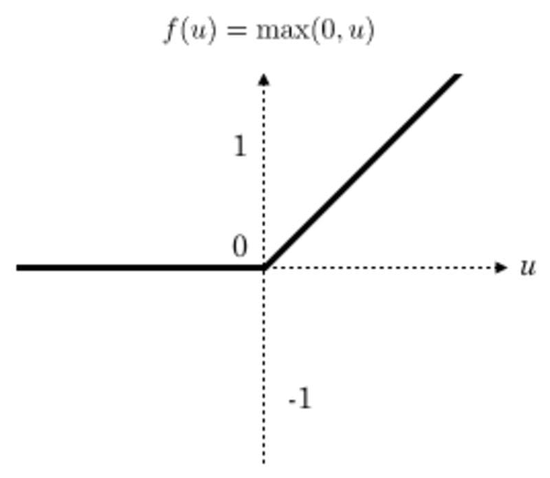
ReLu function plot
Pooling
In this operation, the size of the feature map is reduced further. There are various pooling methods.
A common technique is max-pooling. The size of the pooling filter is usually a 2 by 2 matrix. In max-pooling, the 2 by 2 filter slides over the feature map and picks the largest value in a given box. This operation results in a pooled feature map.
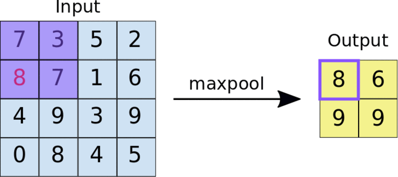
Applying a 2 by 2 pooling filter to a 4 by 4 feature map.
Pooling forces the network to identify key features in the image irrespective of their location. The reduced image size also makes training the network faster.
Dropout Regularization
Applying Dropout Regularization is a common practice in CNNs. This involves randomly dropping some nodes in layers so that they are not updated during back-propagation. This prevents overfitting.
Flattening
Flattening involves transforming the pooled feature map into a single column that is passed to the fully connected layer. This is a common practice during the transition from convolutional layers to fully connected layers.
Fully connected layers
The flattened feature map is then passed to a fully connected layer. There might be several fully connected layers depending on the problem and the network. The last fully connected layer is responsible for outputting the prediction.
An activation function is used in the final layer depending on the type of problem. A sigmoid activation is used for binary classification, while a softmax activation function is used for multi-class image classification.
Fully connected convolutional neural network
Why ConvNets Over Feed-forward Neural Nets?
Having learned about CNNs, you might be wondering why we can’t use normal neural networks for image problems. Normal neural networks can’t extract complex features from images as CNNs can.
The ability of CNNs to extra features from images through the application of filters makes them a better fit for image problems. Also, feeding images directly into the feed-forward neural networks would be computationally expensive.
Convolutional Neural Network Architectures
You can always design your CNNs from scratch. However, you can also take advantage of numerous architectures that have been developed and released publicly. Some of these networks also come with pre-trained models that you can easily adapt for your use case. Some popular architectures include:
You can start using these architectures through Keras applications. For example, here is how to use VGG19:
from tensorflow.keras.applications.vgg19 import VGG19
from tensorflow.keras.preprocessing import image
from tensorflow.keras.applications.vgg16 import preprocess_input
import numpy as np

model = VGG19(weights='imagenet', include_top=False)

img_path = 'elephant.jpg'
img = image.load_img(img_path, target_size=(224, 224))
x = image.img_to_array(img)
x = np.expand_dims(x, axis=0)
x = preprocess_input(x)

features = model.predict(x)
Convolutional Neural Networks (CNN) In TensorFlow Example
Let’s now build a food classification CNN using a food dataset. The dataset contains over a hundred thousand images belonging to 101 classes.
Loading the images
The first step is to download and extract the data.
!wget --no-check-certificate \
    http://data.vision.ee.ethz.ch/cvl/food-101.tar.gz \
    -O food.tar.gz
!tar xzvf food.tar.gz
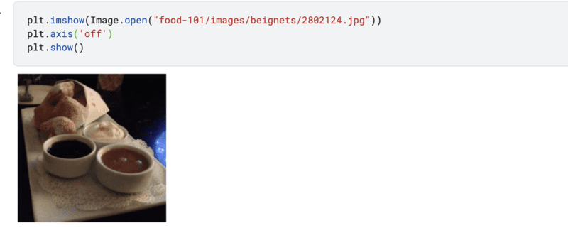
Let’s take a look at one image from the dataset.
plt.imshow(Image.open("food-101/images/beignets/2802124.jpg"))
plt.axis('off')
plt.show()
Generate a tf.data.Dataset
Next, load the images into a TensorFlow dataset. We’ll use 20% of the data for testing and the rest for training. Therefore, we have to create an `ImageDataGenerator` for the training and testing set.
The training set generator will also specify a couple of image augmentation techniques, such as zooming and flipping the images. Augmentation prevents overfitting in the network.
base_dir = 'food-101/images'
train_datagen = ImageDataGenerator(rescale=1./255,
                                   shear_range=0.2,
                                   zoom_range=0.2,
                                   horizontal_flip=True,
                                   width_shift_range=0.1,
                                   height_shift_range=0.1,
                                   validation_split=0.2
                                   )
validation_gen = ImageDataGenerator(rescale=1./255,validation_split=0.2)
With the generators at hand, the next step is to use them to load the food images from the base directory. While loading the images, we specify the target size of the images. All images will be resized to the specified size.
image_size = (200, 200)
training_set = train_datagen.flow_from_directory(base_dir,
                                                 seed=101,
                                                 target_size=image_size,
                                                 batch_size=32,
                                                 subset = "training",
                                                 class_mode='categorical')
When loading the images we also specify:
- The directory where the images are being loaded from.
- The batch size, in this case 32, meaning that the images will be loaded in batches of 32.
- The subset; whether it’s training or validation.
- The class mode as categorical since we have multiple classes. In the case of two classes this would be binary.
validation_set = validation_gen.flow_from_directory(base_dir,
                                               target_size=image_size,
                                               batch_size=32,
                                               subset = "validation",
                                               class_mode='categorical')
Model definition
The next step is to define the CNN model. The architecture of the network will look like the steps we discussed in the how CNNs work section. We’ll use the Keras Sequential API to define the network. CNNs are defined using the Conv2D layer.
model = Sequential([

    Conv2D(filters=32,kernel_size=(3,3),  input_shape = (200, 200, 3),activation='relu'),
    MaxPooling2D(pool_size=(2,2)),

    Conv2D(filters=32,kernel_size=(3,3), activation='relu'),
    MaxPooling2D(pool_size=(2,2)),
    Dropout(0.25),

    Conv2D(filters=64,kernel_size=(3,3), activation='relu'),
    MaxPooling2D(pool_size=(2,2)),
    Dropout(0.25),

    Flatten(),
    Dense(128, activation='relu'),
    Dropout(0.25),
    Dense(101, activation='softmax')
])
The Conv2D layer expects:
- The number of filters to be applied, in this case, 32.
- The size of the kernel, in this case, 3 by 3.
- The size of the input images. 200 by 200 is the size of the image and 3 indicates that it’s a colored image.
- The activation function; usually ReLu.
In the network, we apply pooling with a filter of 2 by 2 and apply a Dropout layer to prevent overfitting.
The final layer has 101 units because there are 101 food classes. The activation function is softmax because it is a multiclass image classification problem.
Compiling the CNN model
We compile the network using categorical loss and accuracy because it involves multiples classes.
model.compile(optimizer='adam',
              loss=keras.losses.CategoricalCrossentropy(),
              metrics=[keras.metrics.CategoricalAccuracy()])
Training the CNN model
Let’s now train the CNN model. We apply the EarlyStopping callback in the training process so that training stops if the model doesn’t improve after a number of iterations. In this case 3 epochs.
callback = EarlyStopping(monitor='loss', patience=3)
history = model.fit(training_set,validation_data=validation_set, epochs=100,callbacks=[callback])
The image dataset we are working with here is quite large. We therefore need to use GPUs to train this model. Let’s utilize free GPUs offered by Layer to train the model. To do that, we need to bundle all the code we have developed above into a single function. This function should return a model. In this case, a TensorFlow model.
To use GPUs to train the model, just decorate the function with a GPU environment. This is specified using the fabric decorator.
#pip install layer-sdk -qqq
import layer
from layer.decorators import model, fabric,pip_requirements
# Authenticate a Layer account
# The trained model will be saved there.
layer.login()
# Initialize a project, the trained model will be save under this project.
layer.init("image-classification")
@pip_requirements(packages=["wget","tensorflow","keras"])
@fabric("f-gpu-small")
@model(name="food-vision")
def train():
    from tensorflow.keras.preprocessing.image import ImageDataGenerator
    import tensorflow as tf
    from tensorflow import keras
    from tensorflow.keras import Sequential
    from tensorflow.keras.layers import Dense,Conv2D,MaxPooling2D,Flatten,Dropout
    from tensorflow.keras.preprocessing.image import ImageDataGenerator
    from tensorflow.keras.callbacks import EarlyStopping
    import os
    import matplotlib.pyplot as plt
    from PIL import Image
    import numpy as np
    import pandas as pd
    import tarfile
    import wget
    wget.download("http://data.vision.ee.ethz.ch/cvl/food-101.tar.gz")
    food_tar = tarfile.open('food-101.tar.gz')
    food_tar.extractall('.')
    food_tar.close()
    plt.imshow(Image.open("food-101/images/beignets/2802124.jpg"))
    plt.axis('off')
    layer.log({"Sample image":plt.gcf()})
    base_dir = 'food-101/images'
    class_names = os.listdir(base_dir)
    train_datagen = ImageDataGenerator(rescale=1./255,
                                   shear_range=0.2,
                                   zoom_range=0.2,
                                   horizontal_flip=True,
                                   width_shift_range=0.1,
                                   height_shift_range=0.1,
                                   validation_split=0.2
                                   )
    validation_gen = ImageDataGenerator(rescale=1./255,validation_split=0.2)
    image_size = (200, 200)
    training_set = train_datagen.flow_from_directory(base_dir,
                                                 seed=101,
                                                 target_size=image_size,
                                                 batch_size=32,
                                                 subset = "training",
                                                 class_mode='categorical')
    validation_set = validation_gen.flow_from_directory(base_dir,
                                               target_size=image_size,
                                               batch_size=32,
                                               subset = "validation",
                                               class_mode='categorical')
    model = Sequential([

    Conv2D(filters=32,kernel_size=(3,3),  input_shape = (200, 200, 3),activation='relu'),
    MaxPooling2D(pool_size=(2,2)),

    Conv2D(filters=32,kernel_size=(3,3), activation='relu'),
    MaxPooling2D(pool_size=(2,2)),
    Dropout(0.25),

    Conv2D(filters=64,kernel_size=(3,3), activation='relu'),
    MaxPooling2D(pool_size=(2,2)),
    Dropout(0.25),

    Flatten(),
    Dense(128, activation='relu'),
    Dropout(0.25),
    Dense(101, activation='softmax')])
    model.compile(optimizer='adam',
              loss=keras.losses.CategoricalCrossentropy(),
              metrics=[keras.metrics.CategoricalAccuracy()])
    callback = EarlyStopping(monitor='loss', patience=3)
    epochs=20
    history = model.fit(training_set,validation_data=validation_set, epochs=epochs,callbacks=[callback])
    metrics_df = pd.DataFrame(history.history)
    layer.log({"Metrics":metrics_df})
    loss, accuracy = model.evaluate(validation_set)
    layer.log({"Accuracy on test dataset":accuracy})
    metrics_df[["loss","val_loss"]].plot()
    layer.log({"Loss plot":plt.gcf()})
    metrics_df[["categorical_accuracy","val_categorical_accuracy"]].plot()
    layer.log({"Accuracy plot":plt.gcf()})
    return model
Training the model is done by passing the training function to the `layer.run` function. If you wish to train the model on your local infrastructure, call the `train()` function normally.
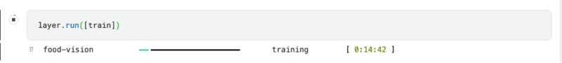
layer.run([train])
Making predictions
With the model ready, we can make predictions on a new image. This can be done in the following steps:
- Fetch the trained model from Layer.
- Loading the image of the same size as the one used in the training images.
- Convert the image into an array.
- Transform the numbers in the array to be between 0 and 1 by dividing by 255. The training images were of the same form.
- Expand the dimensions of the image to add a batch size of 1, since we are making predictions on a single image.
from keras.preprocessing import image
import numpy as np
image_model = layer.get_model('layer/image-classification/models/food-vision').get_train()
!wget --no-check-certificate \
https://upload.wikimedia.org/wikipedia/commons/b/b1/Buttermilk_Beignets_%284515741642%29.jpg \
    -O /tmp/Buttermilk_Beignets_.jpg
test_image = image.load_img('/tmp/Buttermilk_Beignets_.jpg', target_size=(200, 200))
test_image = image.img_to_array(test_image)

test_image = test_image / 255.0
test_image = np.expand_dims(test_image, axis=0)

prediction = image_model.predict(test_image)

prediction[0][0]
Since this is a multiclass network, we’ll use the softmax function to interpret the results. The function converts the logits to a probability for each class.
class_names = os.listdir(base_dir)
scores = tf.nn.softmax(prediction[0])
scores = scores.numpy()
f"{class_names[np.argmax(scores)]} with a { (100 * np.max(scores)).round(2) } percent confidence."
Final Thoughts
In this article, we have covered CNNs at length. Specifically, we talked about:
- What are CNNs?
- How CNNs work.
- CNN architectures.
- How to build a CNN for an image classification problem.
Resources
Derrick Mwiti is experienced in data science, machine learning, and deep learning with a keen eye for building machine learning communities.