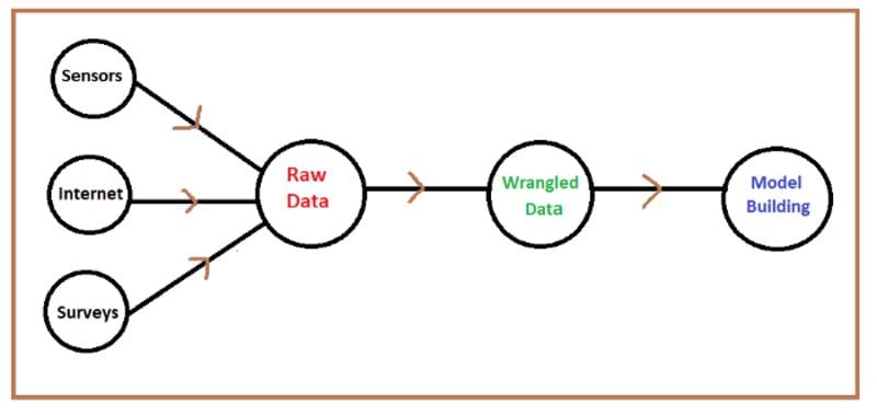
Illustration of stages involved in collecting, cleaning, transforming, and analyzing data. Image by Author.

Key takeaways

• In today’s world driven by information technology, data is now produced at an unprecedented amount
• To fully extract the power of data, data must be collected, processed, transformed, and analyzed to harness its power. 

 
Data is now considered a new kind of gold. The amount of data produced on a daily basis is unprecedented. While raw data is useful, the real power of data comes from data that has been refined, cleaned, transformed, and analyzed using different methods such as descriptive, predictive, and prescriptive analysis, as will be discussed in this article. 

Step 1. Raw Data And Its Sources

 
Raw data could be obtained from several sources such as from sensors, the Internet, or from surveys. Raw data often contains several imperfections that affect its quality as outlined below.

Wrong Data: Data collection can produce errors at different levels. For instance, a survey could be designed for collecting data. However, individuals participating in the survey may not always provide the right information. For example, a participant may enter the wrong information about their age, height, marital status, or income. Error in data collection could also occur when there is an error in the system designed for recording and collecting the data. For instance, a faulty sensor in a thermometer could cause the thermometer to record erroneous temperature data. Human error can also contribute to data collection error, for example, a technician could read an instrument wrongly during data collection.

Since surveys are typically randomized, it is almost impossible to prevent participants from providing false data. Errors from data collected using instruments can be reduced by performing periodic quality assurance checks on the measuring instruments to ensure they are functioning at an optimal level. Human error in reading results from an instrument can be reduced by having second technician or personnel to double-check the readings.

Missing Data: Most datasets contain missing values. The easiest way to deal with missing data is simply to throw away the data point. However, the removal of samples or dropping of entire feature columns is simply not feasible, because we might lose too much valuable data. In this case, we can use different interpolation techniques to estimate the missing values from the other training samples in our dataset. One of the most common interpolation techniques is mean imputation, where we simply replace the missing value by the mean value of the entire feature column. Other options for imputing missing values are median or most frequent (mode), where the latter replaces the missing values by the most frequent values. Whatever imputation method you employ in your model, you have to keep in mind that imputation is only an approximation, and hence can produce an error in the final model. If the data supplied was already preprocessed, you would have to find out how missing values were taken into account. What percentage of the original data was discarded? What imputation method was used to estimate missing values?

Outliers in Data: An outlier is a data point that is very different from the rest of the dataset. Outliers are often just bad data, e.g., due to a malfunctioned sensor; contaminated experiments; or human error in recording data. Sometimes, outliers could indicate something real such as a malfunction in a system. Outliers are very common and are expected in large datasets. Outliers can significantly degrade the predictive power of a machine learning model. A common way to deal with outliers is to simply omit the data points. However, removing real data outliers can be too optimistic, leading to non-realistic models. 

Redundancy in Data: Large datasets with hundreds or thousands of features often lead to redundancy especially when features are correlated with each other. Training a model on a high-dimensional dataset having too many features can sometimes lead to overfitting (model captures both real and random effects). Also, an overly-complex model having too many features can be hard to interpret. One way to solve the problem of redundancy is via feature selection and dimensionality reduction techniques such as PCA (principal component analysis).

Unbalanced Data: An unbalanced data occurs when data proportions for different categories in the dataset are not equal. An example of an unbalanced dataset can be demonstrated using the heights dataset.

  
import numpy as np import pandas as pd
df = pd.read_csv(“heights.csv”)
plt.figure()
sns.countplot(x=”sex”, data = df)
plt.show

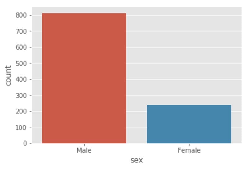
Figure 1. Distribution of dataset. N=1050: 812 (male) and 238 (female) heights. This shows that we have a very unbalanced dataset, with 77% male heights, and 23% female heights. Image by Author.

From Figure 1, we observe that the dataset is not uniform across the Male and Female categories. If one was interested in calculating the average height for the data, this would give a value that is skewed towards the Male average height. One way to deal with this is to calculate the average height for each category, as shown in Figure 2. 

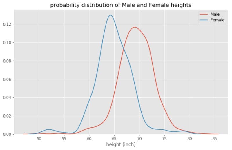
Figure 2. The distribution of male and female heights. Image by Author.

Lack of Variability in Data: A dataset lacks variability when it contains too few features that it doesn’t represent the whole picture. For example, a dataset for predicting the price of a house based on square footage only lacks variability. The best way to resolve this problem is to include more representative features such as the number of bedrooms, the number of bathrooms, year built, lot size, HOA fees, zip code, etc.

Dynamic Data: In this case, the data is not static, but it depends on time and is changing each time, e.g., stock data. In this case, time-dependent analytic tools such as time-series analysis should be used for analyzing the dataset and for predictive modeling (forecasting).

Size of Data: In this case, the size of the sample data may be too small that it is not representative of the whole population. This can be resolved by ensuring that the sample dataset is large enough and representative of the population. A large sample containing a large number of observations will reduce variance error (variance error decreases with sample size according to the Central Limit Theorem). The main drawback with larger samples is that collecting the data may require a lot of time. Also, building a machine learning model with very large datasets can be computationally very costly in terms of computing time (time required for training and testing the model).

Step 2. Data Wrangling

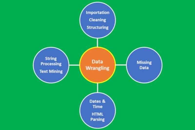
Figure 3: Data wrangling process. Image by Author

Data wrangling is the process of converting data from its raw form to a tidy form ready for analysis. Data wrangling is an important step in data preprocessing and includes several processes like data importing, data cleaning, data structuring, string processing, HTML parsing, handling dates and times, handling missing data, and text mining.

The process of data wrangling is a critical step for any data scientist. Very rarely is data easily accessible in a data science project for analysis. It is more likely for the data to be in a file, a database, or extracted from documents such as web pages, tweets, or PDFs. Knowing how to wrangle and clean data will enable you to derive critical insights from your data that would otherwise be hidden.

Step 3. Data Analysis

After raw data has been cleaned, processed, and transformed, the final and most important step is to analyze the data. We will discuss 3 classes of data analysis techniques, namely, descriptive analysis, predictive analysis, and predictive analysis.

(i) Descriptive Data Analysis

 
This involves the use of data for story telling or data visualization using barplots, line graphs, histograms, scatter plots, pairplots, density plots, qqplots, etc. Some of the most common packages for descriptive data analysis include

• Matplotlib
• Ggplot2
• Seaborn

(ii) Predictive Data Analysis

 
This involves the use of data for building predictive models that could be used for making predictions on unseen data. Some of the most common packages for predictive analytics include

• Sci-kit learn package
• Caret package
• Tensorflow

Predictive data analysis can be further classified into the following groups:

a) Supervised Learning (Continuous Variable Prediction)

• Basic regression
• Multi-regression analysis

b) Supervised Learning (Discrete Variable Prediction)

• Logistic Regression Classifier
• Support Vector Machine Classifier
• K-nearest neighbor (KNN) Classifier
• Decision Tree Classifier
• Random Forest Classifier

c) Unsupervised Learning

• Kmeans clustering algorithm

(iii) Prescriptive Data Analysis

 
This involves the use of data for building models that can be used for prescribing a course of action based on insights derived from data. Some prescriptive data analysis techniques include

• Probabilistic modeling
• Optimization methods and operations research
• Monte-Carlo simulations

Summary

 
Even though data is now produced at an unprecedented amount, data must be collected, processed, transformed, and analyzed to harness its power. We’ve discussed the 3 main stages involved: Raw Data and Its Sources; Wrangling of Raw Data; and Data Analysis.

 
 
Benjamin O. Tayo is a Physicist, Data Science Educator, and Writer, as well as the Owner of DataScienceHub. Previously, Benjamin was teaching Engineering and Physics at U. of Central Oklahoma, Grand Canyon U., and Pittsburgh State U.