A Guide for Customer Retention Analysis with SQL

comments

By Luba Belokon, Statsbot

Whether you’re selling groceries, financial services, or gym memberships, successful recruitment of new customers is only truly successful if they return to buy from you again. The metric which reflects this is called retention, and the approach we use is customer retention analysis. It’s one of the key metrics that influences revenue. When your customers’ retention is law, you’ll spend all of the income from your business on marketing.

At the same time, retention is easy to improve if you can calculate it the right way using SQL and your database. In this post, we’ll guide you step by step on how to make basic customer retention analysis, how to build customer retention over time, new vs. existing customers retention curves, and how to calculate retention analysis in cohorts.

Basic customer retention curves

 
Customer retention curves are essential to any business looking to understand its clients, and will go a long way towards explaining other things like sales figures or the impact of marketing initiatives. They are an easy way to visualize a key interaction between customers and the business, which is to say, whether or not customers return — and at what rate — after the first visit.

The first step to building a customer retention curve is to identify those who visited your business during the reference period, what I will call p1. It is important that the length of the period chosen is a reasonable one, and reflects expected frequency of visits.

Different types of businesses are going to expect their customers to return at different rates:

• A coffee shop may choose to use an expected frequency of visits of once a week.
• A supermarket may choose a longer period, perhaps 2 weeks or a month.

In the following example, I will use a month, and assume that we are looking at customer retention of customers who visited in January 2016 over the following year.

As previously stated, the first step is to identify the original pool of customers:

January_pool AS

(                
                SELECT DISTINCT cust_id

                FROM            dataset

                WHERE           month(transaction_date)=1

                AND             year(transaction_date)=2016)

Then, we look at how those customers behaved over time: for example, how many of them returned per month over the rest of the year?

SELECT Year(transaction_date),
       Month(transaction_date),
       count (distinct cust_id) AS number

FROM dataset

WHERE year(transaction_date)=2016

AND cust_id IN january_pool

GROUP BY 1,

         2

As you can see, the original SELECT function is included in this second step.

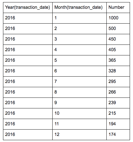
If we had 1000 unique customers in January, we can expect our results to look something like this:

The resulting graph would then look like this:

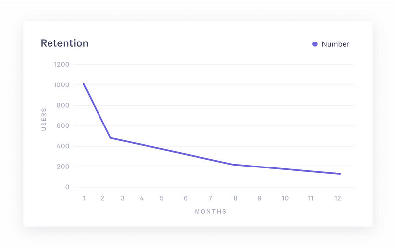
Data visualized with Statsbot

Evolution of customer retention over time

 
What is described above is obviously only the first step, as we would also like to see whether there are any trends in customer retention, i.e. are we getting any better at it?

So, one idea we might have is to say: of those who came in January, how many returned in February? Of those who came in February, how many returned in March? And other one-month intervals.

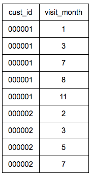
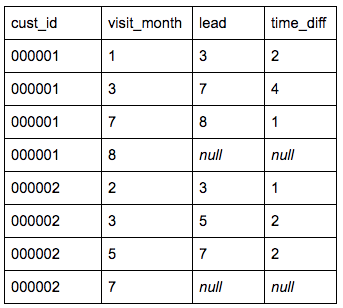
So, then we need to set up an iterative model, which can be built in a few simple steps. First, we need to create a table where each user’s visits are logged by month, allowing for the possibility that these will have occurred over multiple years since whenever our business started operations. I have assumed here that the start date is the year 2000, but you can adjust this as necessary.

Visit_log AS

SELECT cust_id,

       datediff(month, ‘2000–01–01’, transaction_date) AS visit_month

FROM dataset

GROUP BY 1,

         2

ORDER BY 1,

         2

This will give us a view that looks like this:

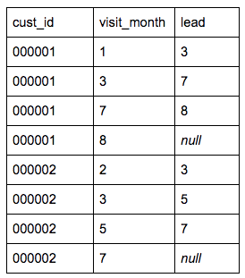
We then need to reorganize this information in order to identify the time lapse between each visit. So, for each person and for each month, see when the next visit is.

Time_lapse AS

    SELECT cust_id,

           visit_month lead(visit_month, 1) over (partition BY cust_id ORDER BY cust_id, visit_month)

    FROM visit_log

We then need to calculate the time gaps between visits:

Time_diff_calculated AS

    SELECT cust_id,

           visit_month,

           lead,

           lead — visit_month AS time_diff

    FROM time_lapse

Now, a small reminder of what customer retention analysis measures: it is the proportion of customers who return after x lag of time. So, what we want to do is compare the number of customers visiting in a given month to how many of those return the next month. We also want to define those who return after a certain absence, and those who don’t return at all. In order to do that, we need to categorize the customers depending on their visit pattern.

Custs_categorized AS

SELECT cust_id,

       visit_month,

       CASE

             WHEN time_diff=1 THEN ‘retained’,

             WHEN time_diff>1 THEN ‘lagger’,

             WHEN time_diff IS NULL THEN ‘lost’

       END AS cust_type

FROM time_diff_calculated

This will allow us, in a final step, to establish a count of the number of customers who visited in a given month, and how many of those return the next month.

SELECT visit_month,

       count(cust_id where cust_type=’retained’)/count(cust_id) AS retention

FROM custs_categorized

GROUP BY 1

This gives us, month by month, the proportion of customers who returned.

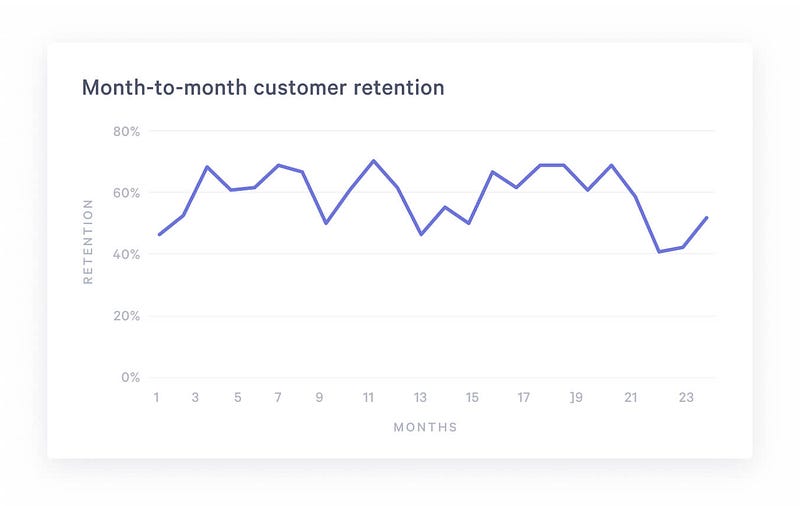
Data visualized with Statsbot