Getting Started with TensorFlow: A Machine Learning Tutorial

comments

By Dino Causevic, Toptal.

TensorFlow is an open source software library created by Google that is used to implement machine learning and deep learning systems. These two names contain a series of powerful algorithms that share a common challenge—to allow a computer to learn how to automatically spot complex patterns and/or to make best possible decisions.

If you’re interested in details about these systems, you can learn more from the Toptal blog posts on machine learning and deep learning.

TensorFlow, at its heart, is a library for dataflow programming. It leverages various optimization techniques to make the calculation of mathematical expressions easier and more performant.

Some of the key features of TensorFlow are:

• Efficiently works with mathematical expressions involving multi-dimensional arrays
• Good support of deep neural networks and machine learning concepts
• GPU/CPU computing where the same code can be executed on both architectures
• High scalability of computation across machines and huge data sets

Together, these features make TensorFlow the perfect framework for machine intelligence at a production scale.

In this TensorFlow tutorial, you will learn how you can use simple yet powerful machine learning methods in TensorFlow and how you can use some of its auxiliary libraries to debug, visualize, and tweak the models created with it.

Installing TensorFlow
We will be using the TensorFlow Python API, which works with Python 2.7 and Python 3.3+. The GPU version (Linux only) requires the Cuda Toolkit 7.0+ and cuDNN v2+.

We shall use the Conda package dependency management system to install TensorFlow. Conda allows us to separate multiple environments on a machine. You can learn how to install Conda from here.

After installing Conda, we can create the environment that we will use for TensorFlow installation and use. The following command will create our environment with some additional libraries like NumPy, which is very useful once we start to use TensorFlow.

The Python version installed inside this environment is 2.7, and we will use this version in this article.

conda create --name TensorflowEnv biopython

To make things easy, we are installing biopython here instead of just NumPy. This includes NumPy and a few other packages that we will be needing. You can always install the packages as you need them using the conda install or the pip install commands.

The following command will activate the created Conda environment. We will be able to use packages installed within it, without mixing with packages that are installed globally or in some other environments.

source activate TensorFlowEnv

The pip installation tool is a standard part of a Conda environment. We will use it to install the TensorFlow library. Prior to doing that, a good first step is updating pip to the latest version, using the following command:

pip install --upgrade pip

Now we are ready to install TensorFlow, by running:

pip install tensorflow

The download and build of TensorFlow can take several minutes. At the time of writing, this installs TensorFlow 1.1.0.

Data Flow Graphs

In TensorFlow, computation is described using data flow graphs. Each node of the graph represents an instance of a mathematical operation (like addition, division, or multiplication) and each edge is a multi-dimensional data set (tensor) on which the operations are performed.

As TensorFlow works with computational graphs, they are managed where each node represents the instantiation of an operation where each operation has zero or more inputs and zero or more outputs.

Edges in TensorFlow can be grouped in two categories: Normal edges transfer data structure (tensors) where it is possible that the output of one operation becomes the input for another operation and special edges, which are used to control dependency between two nodes to set the order of operation where one node waits for another to finish.

Simple Expressions

Before we move on to discuss elements of TensorFlow, we will first do a session of working with TensorFlow, to get a feeling of what a TensorFlow program looks like.

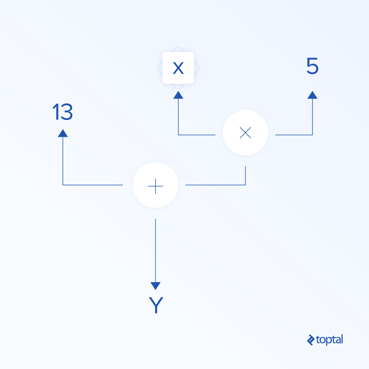
Let’s start with simple expressions and assume that, for some reason, we want to evaluate the function y = 5*x + 13 in TensorFlow fashion.

In simple Python code, it would look like:

x = -2.0
y = 5*x + 13
print y

which gives us in this case a result of 3.0.

Now we will convert the above expression into TensorFlow terms.

Constants

In TensorFlow, constants are created using the function constant, which has the signature constant(value, dtype=None, shape=None, name='Const', verify_shape=False), where value is an actual constant value which will be used in further computation, dtype is the data type parameter (e.g., float32/64, int8/16, etc.), shape is optional dimensions, name is an optional name for the tensor, and the last parameter is a boolean which indicates verification of the shape of values.

If you need constants with specific values inside your training model, then the constant object can be used as in following example:

z = tf.constant(5.2, name="x", dtype=tf.float32)

Variables

Variables in TensorFlow are in-memory buffers containing tensors which have to be explicitly initialized and used in-graph to maintain state across session. By simply calling the constructor the variable is added in computational graph.

Variables are especially useful once you start with training models, and they are used to hold and update parameters. An initial value passed as an argument of a constructor represents a tensor or object which can be converted or returned as a tensor. That means if we want to fill a variable with some predefined or random values to be used afterwards in the training process and updated over iterations, we can define it in the following way:

k = tf.Variable(tf.zeros([1]), name="k")

Another way to use variables in TensorFlow is in calculations where that variable isn’t trainable and can be defined in the following way:

k = tf.Variable(tf.add(a, b), trainable=False)

Sessions
In order to actually evaluate the nodes, we must run a computational graph within a session.

A session encapsulates the control and state of the TensorFlow runtime. A session without parameters will use the default graph created in the current session, otherwise the session class accepts a graph parameter, which is used in that session to be executed.

Below is a brief code snippet that shows how the terms defined above can be used in TensorFlow to calculate a simple linear function.

import tensorflow as tf

x = tf.constant(-2.0, name="x", dtype=tf.float32)
a = tf.constant(5.0, name="a", dtype=tf.float32)
b = tf.constant(13.0, name="b", dtype=tf.float32)

y = tf.Variable(tf.add(tf.multiply(a, x), b))

init = tf.global_variables_initializer()

with tf.Session() as session:
    session.run(init)
    print session.run(y)

Using TensorFlow: Defining Computational Graphs
The good thing about working with dataflow graphs is that the execution model is separated from its execution (on CPU, GPU, or some combination) where, once implemented, software in TensorFlow can be used on the CPU or GPU where all complexity related to code execution is hidden.

The computation graph can be built in the process of using the TensorFlow library without having to explicitly instantiate Graph objects.

A Graph object in TensorFlow can be created as a result of a simple line of code like c = tf.add(a, b). This will create an operation node that takes two tensors a and b that produce their sum c as output.

The computation graph is a built-in process that uses the library without needing to call the graph object directly. A graph object in TensorFlow, which contains a set of operations and tensors as units of data, is used between operations which allows the same process and contains more than one graph where each graph will be assigned to a different session. For example, the simple line of code c = tf.add(a, b) will create an operation node that takes two tensors a and b as input and produces their sum c as output.

TensorFlow also provides a feed mechanism for patching a tensor to any operation in the graph, where the feed replaces the output of an operation with the tensor value. The feed data are passed as an argument in the run() function call.

A placeholder is TensorFlow’s way of allowing developers to inject data into the computation graph through placeholders which are bound inside some expressions. The signature of the placeholder is:

placeholder(dtype, shape=None, name=None)

where dtype is the type of elements in the tensors and can provide both the shape of the tensors to be fed and the name for the operation.

If the shape isn’t passed, this tensor can be fed with any shape. An important note is that the placeholder tensor has to be fed with data, otherwise, upon execution of the session and if that part is missing, the placeholder generates an error with the following structure:

InvalidArgumentError (see above for traceback): You must feed a value for placeholder tensor 'y' with dtype float

The advantage of placeholders is that they allow developers to create operations, and the computational graph in general, without needing to provide the data in advance for that, and the data can be added in runtime from external sources.

Let’s take a simple problem of multiplying two integers x and y in TensorFlow fashion, where a placeholder will be used together with a feed mechanism through the session run method.

import tensorflow as tf

x = tf.placeholder(tf.float32, name="x")
y = tf.placeholder(tf.float32, name="y")

z = tf.multiply(x, y, name="z")

with tf.Session() as session:
    print session.run(z, feed_dict={x: 2.1, y: 3.0})

Visualizing the Computational Graph with TensorBoard
TensorBoard is a visualization tool for analyzing data flow graphs. This can be useful for gaining better understanding of machine learning models.

With TensorBoard, you can gain insight into different types of statistics about the parameters and details about the parts of the computational graph in general. It is not unusual that a deep neural network has large number of nodes. TensorBoard allows developers to get insight into each node and how the computation is executed over the TensorFlow runtime.

Now let’s get back to our example from the beginning of this TensorFlow tutorial where we defined a linear function with the format y = a*x + b.

In order to log events from session which later can be used in TensorBoard, TensorFlow provides the FileWriter class. It can be used to create an event file for storing summaries and events where the constructor accepts six parameters and looks like:

__init__(logdir, graph=None, max_queue=10, flush_secs=120, graph_def=None, filename_suffix=None)

where the logdir parameter is required, and others have default values. The graph parameter will be passed from the session object created in the training program. The full example code looks like:

import tensorflow as tf


x = tf.constant(-2.0, name="x", dtype=tf.float32)
a = tf.constant(5.0, name="a", dtype=tf.float32)
b = tf.constant(13.0, name="b", dtype=tf.float32)


y = tf.Variable(tf.add(tf.multiply(a, x), b))


init = tf.global_variables_initializer()


with tf.Session() as session:
    merged = tf.summary.merge_all() // new
    writer = tf.summary.FileWriter("logs", session.graph) // new


    session.run(init)
    print session.run(y)

We added just two new lines. We merge all the summaries collected in the default graph, and FileWriteris used to dump events to the file as we described above, respectively.

After running the program, we have the file in the directory logs, and the last step is to run tensorboard:

tensorboard --logdir logs/

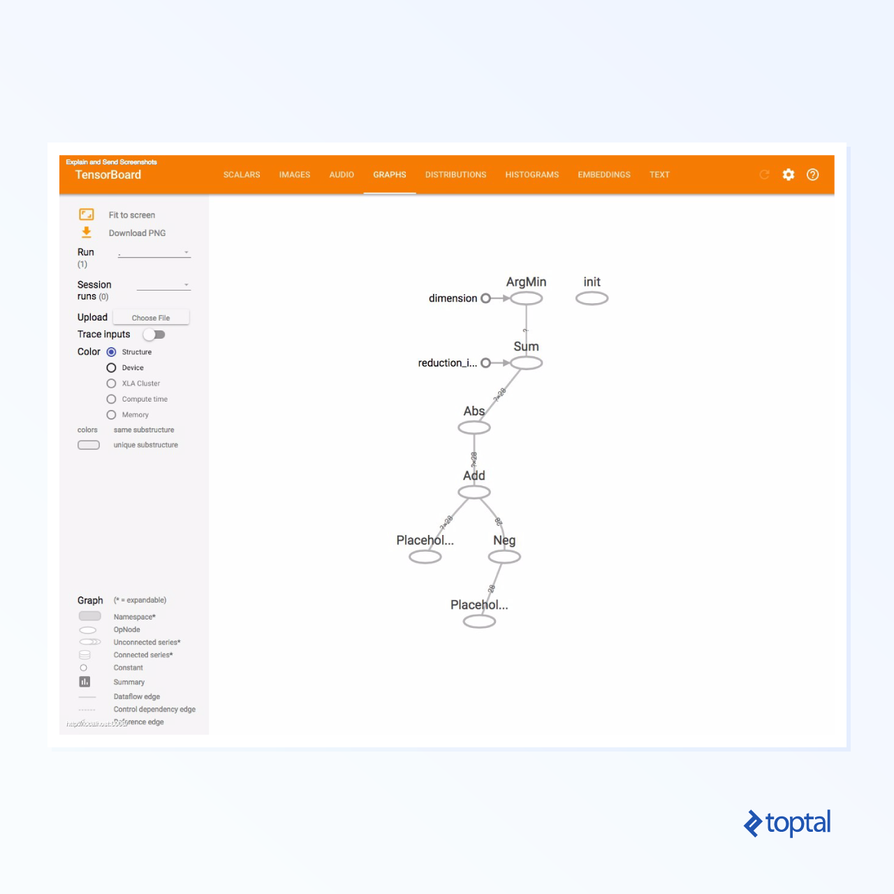
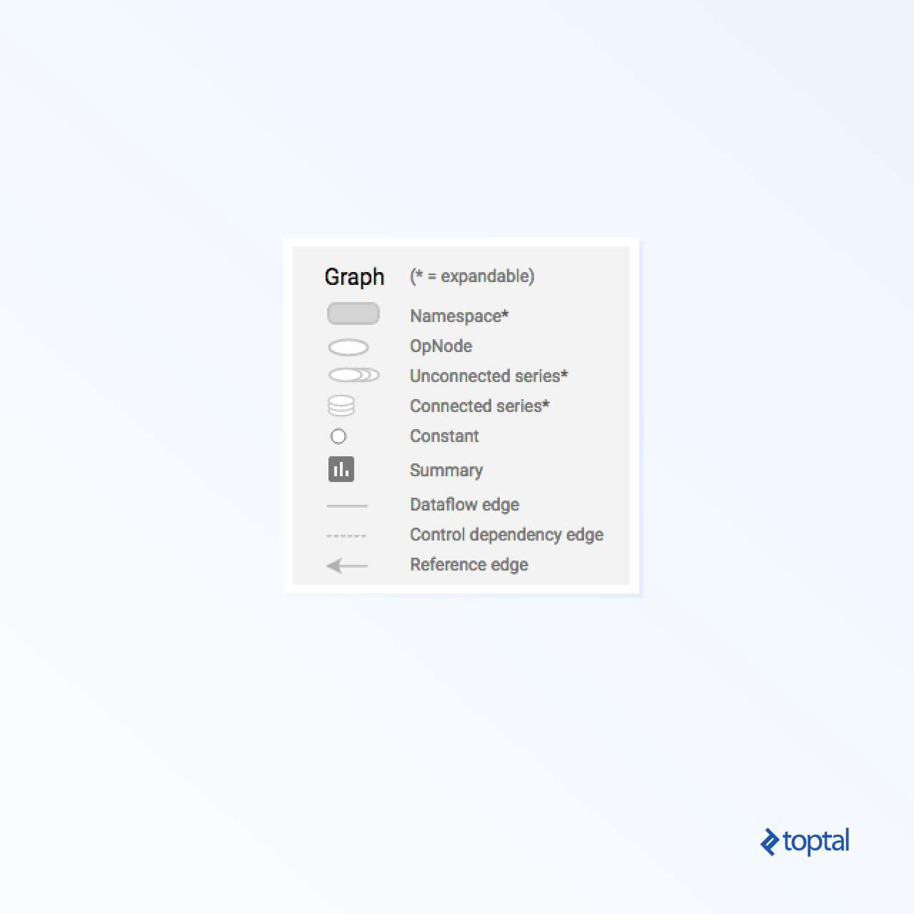
Now TensorBoard is started and running on the default port 6006. After opening https://localhost:6006 and clicking on the Graphs menu item (located at the top of the page), you will be able to see the graph, like the one in the picture below:

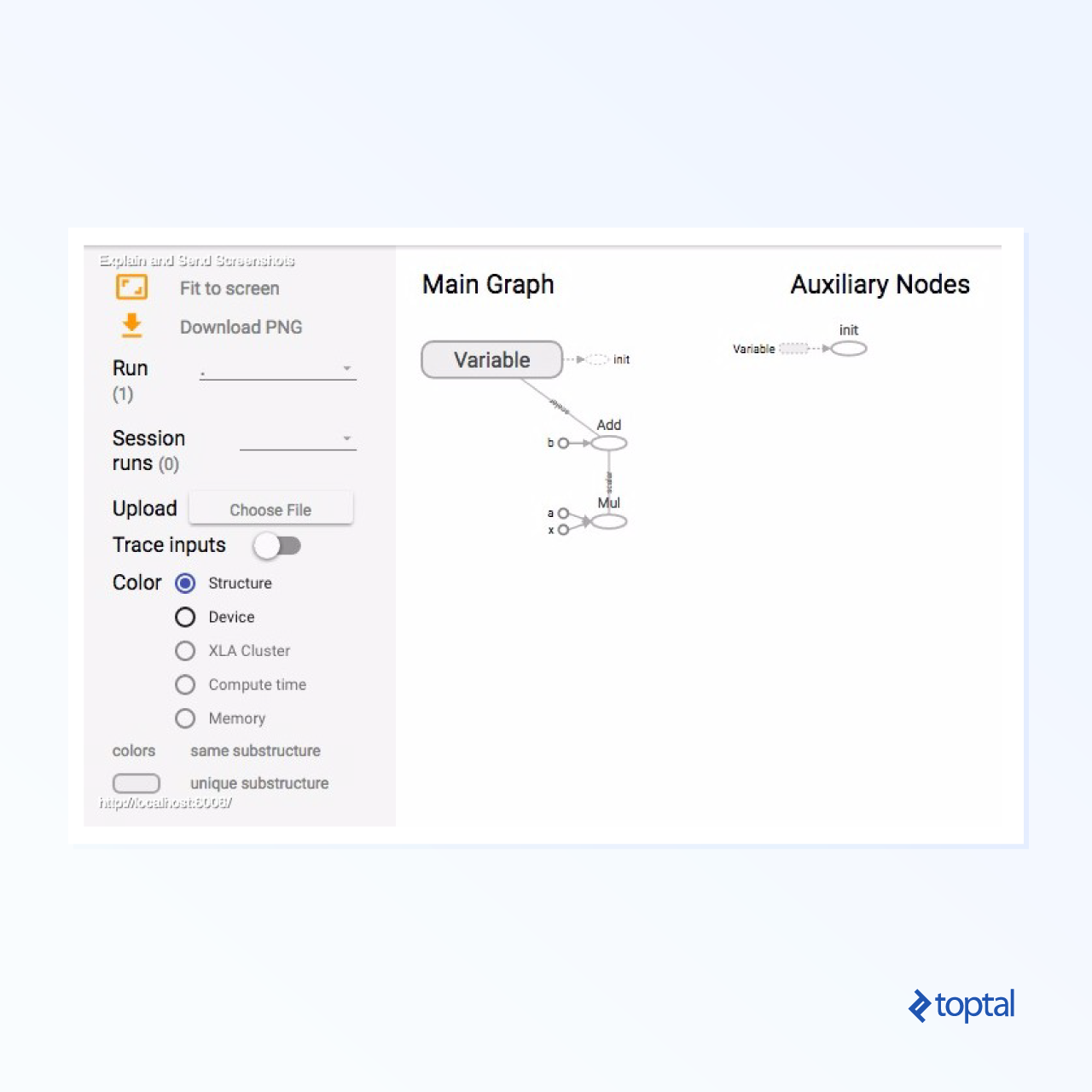
TensorBoard marks constants and summary nodes specific symbols, which are described below.

Mathematics with TensorFlow
Tensors are the basic data structures in TensorFlow, and they represent the connecting edges in a dataflow graph.

A tensor simply identifies a multidimensional array or list. The tensor structure can be identified with three parameters: rank, shape, and type.

• Rank: Identifies the number of dimensions of the tensor. A rank is known as the order or n-dimensions of a tensor, where for example rank 1 tensor is a vector or rank 2 tensor is matrix.
• Shape: The shape of a tensor is the number of rows and columns it has.
• Type: The data type assigned to tensor elements.

To build a tensor in TensorFlow, we can build an n-dimensional array. This can be done easily by using the NumPy library, or by converting a Python n-dimensional array into a TensorFlow tensor.

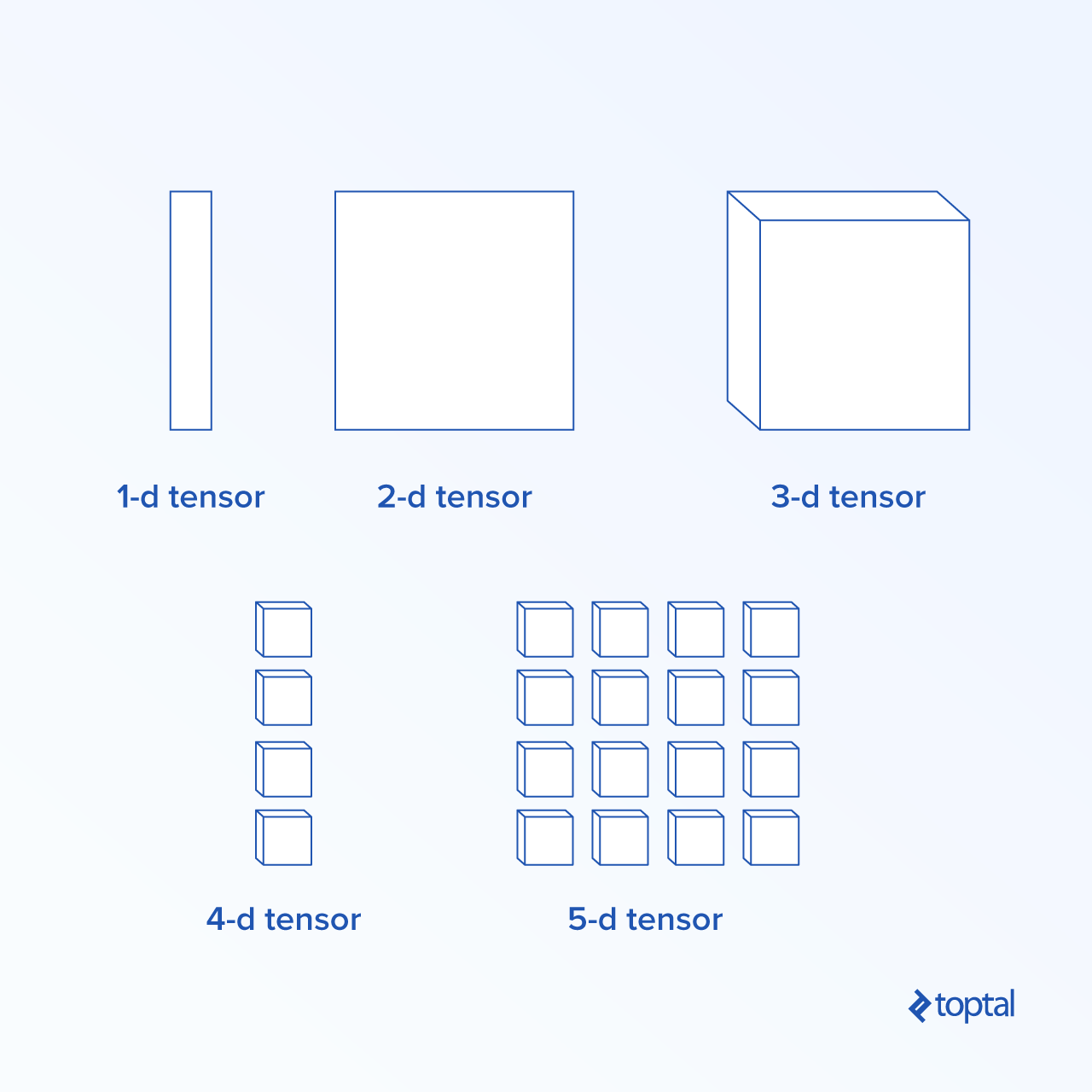
To build a 1-d tensor, we will use a NumPy array, which we’ll construct by passing a built-in Python list.

import numpy as np
tensor_1d = np.array([1.45, -1, 0.2, 102.1])

Working with this kind of array is similar to working with a built-in Python list. The main difference is that the NumPy array also contains some additional properties, like dimension, shape, and type.

>> print tensor_1d
[   1.45   -1.      0.2   102.1 ]

>> print tensor_1d[0]
1.45

>> print tensor_1d[2]
0.2

>> print tensor_1d.ndim
1

>> print tensor_1d.shape
(4,)

>> print tensor_1d.dtype
float64

A NumPy array can be easily converted into a TensorFlow tensor with the auxiliary function convert_to_tensor, which helps developers convert Python objects to tensor objects. This function accepts tensor objects, NumPy arrays, Python lists, and Python scalars.

tensor = tf.convert_to_tensor(tensor_1d, dtype=tf.float64)

Now if we bind our tensor to the TensorFlow session, we will be able to see the results of our conversion.

tensor = tf.convert_to_tensor(tensor_1d, dtype=tf.float64)

with tf.Session() as session:
    print session.run(tensor)
    print session.run(tensor[0])
    print session.run(tensor[1])

Output:

[   1.45   -1.      0.2   102.1 ]
1.45
-1.0

We can create a 2-d tensor, or matrix, in a similar way:

tensor_2d = np.array(np.random.rand(4, 4), dtype='float32')
tensor_2d_1 = np.array(np.random.rand(4, 4), dtype='float32')
tensor_2d_2 = np.array(np.random.rand(4, 4), dtype='float32')

m1 = tf.convert_to_tensor(tensor_2d)
m2 = tf.convert_to_tensor(tensor_2d_1)
m3 = tf.convert_to_tensor(tensor_2d_2)
mat_product = tf.matmul(m1, m2)
mat_sum = tf.add(m2, m3)
mat_det = tf.matrix_determinant(m3)

with tf.Session() as session:
    print session.run(mat_product)
    print session.run(mat_sum)
    print session.run(mat_det)

Tensor Operations
In the example above, we introduce a few TensorFlow operations on the vectors and matrices. The operations perform certain calculations on the tensors. Which calculations those are is shown in the table below.

TensorFlow operations listed in the table above work with tensor objects, and are performed element-wise. So if you want to calculate the cosine for a vector x, the TensorFlow operation will do calculations for each element in the passed tensor.

tensor_1d = np.array([0, 0, 0])
tensor = tf.convert_to_tensor(tensor_1d, dtype=tf.float64)
with tf.Session() as session:
    print session.run(tf.cos(tensor))

Output:

[ 1.  1.  1.]

Matrix Operations

Matrix operations are very important for machine learning models, like linear regression, as they are often used in them. TensorFlow supports all the most common matrix operations, like multiplication, transposing, inversion, calculating the determinant, solving linear equations, and many more.

Next up, we will explain some of the matrix operations. They tend to be important when comes to machine learning models, like in linear regression. Let’s write some code that will do basic matrix operations like multiplication, getting the transpose, getting the determinant, multiplication, sol, and many more.

Below are basic examples of calling these operations.

import tensorflow as tf
import numpy as np

def convert(v, t=tf.float32):
    return tf.convert_to_tensor(v, dtype=t)

m1 = convert(np.array(np.random.rand(4, 4), dtype='float32'))
m2 = convert(np.array(np.random.rand(4, 4), dtype='float32'))
m3 = convert(np.array(np.random.rand(4, 4), dtype='float32'))
m4 = convert(np.array(np.random.rand(4, 4), dtype='float32'))
m5 = convert(np.array(np.random.rand(4, 4), dtype='float32'))

m_tranpose = tf.transpose(m1)
m_mul = tf.matmul(m1, m2)
m_det = tf.matrix_determinant(m3)
m_inv = tf.matrix_inverse(m4)
m_solve = tf.matrix_solve(m5, [[1], [1], [1], [1]])

with tf.Session() as session:
    print session.run(m_tranpose)
    print session.run(m_mul)
    print session.run(m_inv)
    print session.run(m_det)
    print session.run(m_solve)