Regularization in Machine Learning
Regularization is a technique that helps to avoid overfitting and also make a predictive model more understandable.
By Prashant Gupta.
One of the major aspects of training your machine learning model is avoiding overfitting. The model will have a low accuracy if it is overfitting. This happens because your model is trying too hard to capture the noise in your training dataset. By noise we mean the data points that don’t really represent the true properties of your data, but random chance. Learning such data points, makes your model more flexible, at the risk of overfitting.
The concept of balancing bias and variance, is helpful in understanding the phenomenon of overfitting.
One of the ways of avoiding overfitting is using cross validation, that helps in estimating the error over test set, and in deciding what parameters work best for your model.
This article will focus on a technique that helps in avoiding overfitting and also increasing model interpretability.
Regularization
This is a form of regression, that constrains/ regularizes or shrinks the coefficient estimates towards zero. In other words, this technique discourages learning a more complex or flexible model, so as to avoid the risk of overfitting.
A simple relation for linear regression looks like this. Here Y represents the learned relation and β represents the coefficient estimates for different variables or predictors(X).
Y ≈ β0 + β1X1 + β2X2 + … + βpXp
The fitting procedure involves a loss function, known as residual sum of squares or RSS. The coefficients are chosen, such that they minimize this loss function.
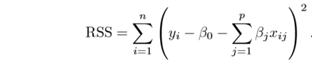
Now, this will adjust the coefficients based on your training data. If there is noise in the training data, then the estimated coefficients won’t generalize well to the future data. This is where regularization comes in and shrinks or regularizes these learned estimates towards zero.
Ridge Regression
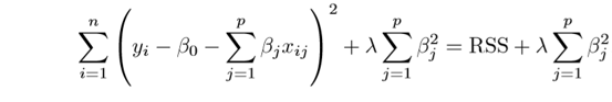
Above image shows ridge regression, where the RSS is modified by adding the shrinkage quantity. Now, the coefficients are estimated by minimizing this function. Here, λ is the tuning parameter that decides how much we want to penalize the flexibility of our model. The increase in flexibility of a model is represented by increase in its coefficients, and if we want to minimize the above function, then these coefficients need to be small. This is how the Ridge regression technique prevents coefficients from rising too high. Also, notice that we shrink the estimated association of each variable with the response, except the intercept β0, This intercept is a measure of the mean value of the response when xi1 = xi2 = …= xip = 0.
When λ = 0, the penalty term has no effect, and the estimates produced by ridge regression will be equal to least squares. However, as λ→∞, the impact of the shrinkage penalty grows, and the ridge regression coefficient estimates will approach zero. As can be seen, selecting a good value of λ is critical. Cross validation comes in handy for this purpose. The coefficient estimates produced by this method are also known as the L2 norm.
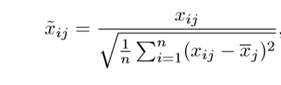
The coefficients that are produced by the standard least squares method are scale equivariant, i.e. if we multiply each input by c then the corresponding coefficients are scaled by a factor of 1/c. Therefore, regardless of how the predictor is scaled, the multiplication of predictor and coefficient(Xjβj) remains the same. However, this is not the case with ridge regression, and therefore, we need to standardize the predictors or bring the predictors to the same scale before performing ridge regression. The formula used to do this is given below.
Lasso
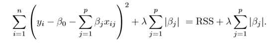
Lasso is another variation, in which the above function is minimized. Its clear that this variation differs from ridge regression only in penalizing the high coefficients. It uses |βj| (modulus)instead of squares of β, as its penalty. In statistics, this is known as the L1 norm.
Lets take a look at above methods with a different perspective. The ridge regression can be thought of as solving an equation, where summation of squares of coefficients is less than or equal to s. And the Lasso can be thought of as an equation where summation of modulus of coefficients is less than or equal to s. Here, s is a constant that exists for each value of shrinkage factor λ. These equations are also referred to as constraint functions.
Consider their are 2 parameters in a given problem. Then according to above formulation, the ridge regression is expressed by β1² + β2² ≤ s. This implies that ridge regression coefficients have the smallest RSS(loss function) for all points that lie within the circle given by β1² + β2² ≤ s.
Similarly, for lasso, the equation becomes,|β1|+|β2|≤ s. This implies that lasso coefficients have the smallest RSS(loss function) for all points that lie within the diamond given by |β1|+|β2|≤ s.
The image below describes these equations.
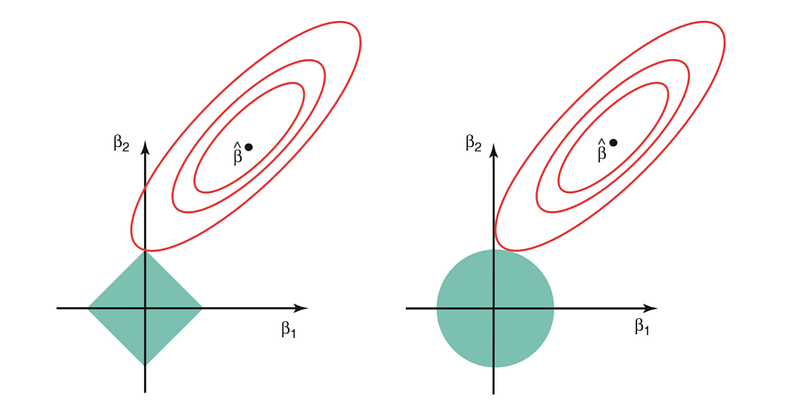
The above image shows the constraint functions(green areas), for lasso (left) and ridge regression (right), along with contours for RSS (red ellipse). Points on the ellipse share the value of RSS. For a very large value of s, the green regions will contain the center of the ellipse, making coefficient estimates of both regression techniques, equal to the least squares estimates. But, this is not the case in the above image. In this case, the lasso and ridge regression coefficient estimates are given by the first point at which an ellipse contacts the constraint region. Since ridge regression has a circular constraint with no sharp points, this intersection will not generally occur on an axis, and so the ridge regression coefficient estimates will be exclusively non-zero.
However, the lasso constraint has corners at each of the axes, and so the ellipse will often intersect the constraint region at an axis. When this occurs, one of the coefficients will equal zero. In higher dimensions(where parameters are much more than 2), many of the coefficient estimates may equal zero simultaneously.
This sheds light on the obvious disadvantage of ridge regression, which is model interpretability. It will shrink the coefficients for least important predictors, very close to zero. But it will never make them exactly zero. In other words, the final model will include all predictors. However, in the case of the lasso, the L1 penalty has the effect of forcing some of the coefficient estimates to be exactly equal to zero when the tuning parameter λ is sufficiently large. Therefore, the lasso method also performs variable selection and is said to yield sparse models.
What does Regularization achieve?
A standard least squares model tends to have some variance in it, i.e. this model won’t generalize well for a data set different than its training data. Regularization, significantly reduces the variance of the model, without substantial increase in its bias. So the tuning parameter λ, used in the regularization techniques described above, controls the impact on bias and variance. As the value of λ rises, it reduces the value of coefficients and thus reducing the variance. Till a point, this increase in λ is beneficial as it is only reducing the variance(hence avoiding overfitting), without loosing any important properties in the data. But after certain value, the model starts loosing important properties, giving rise to bias in the model and thus underfitting. Therefore, the value of λ should be carefully selected.
This is all the basic you will need, to get started with Regularization. It is a useful technique that can help in improving the accuracy of your regression models. A popular library for implementing these algorithms is Scikit-Learn. It has a wonderful API that can get your model up an running with just a few lines of code in python.
If you have any questions, leave a comment and I will do my best to answer.
You can also follow me on Twitter, email me directly or find me on linkedin. I’d love to hear from you.
That’s all folks, Have a nice day :)
Credit
Content for this article is inspired and taken from, An Introduction to Statistical Learning by Gareth James, Daniela Witten, Trevor Hastie, Robert Tibshirani.
Bio: Prashant Gupta is a Machine Learning Engineer, Android Developer, Tech Enthusiast.
Original. Reposted with permission.
Related