How (dis)similar are my train and test data?
This articles examines a scenario where your machine learning model can fail.
By Shikhar Gupta.
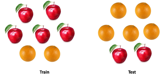
They always say that don’t compare apples to oranges. But how about if we’re comparing one mix of apples and oranges with another mix of apples and oranges, but the distribution is different. Can you still compare ? And how will you go about it ?
In most of the cases in the real world, you’ll come across the latter.
This happens quite often in data science. While developing a machine learning model we come across a situation where our model performs well on our training data but it fails to match up to the same performance for the test data.
I’m not referring to overfitting here. Even if I’ve picked my best model based on cross-validation and it still performs poorly on test data, there is some inherent patterns in test data that we are not capturing.<
Imagine a situation where I’m trying to model the shopping behaviour of customers. Now if my train and test data looks like below then you can clearly see the issue here.
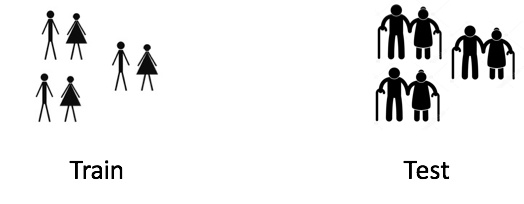
The model will be trained on customers with lower average age compared to test. This model would have never seen age patterns like the ones in test data. If age is an important feature in your model, then it’ll not perform well on the test.
In this post, I’ll talk about how to identify this issue and some raw ideas on how we can fix it.
Covariate Shift
We can define this situation more formally. Covariate refers to the predictor variables in our model. Covariate shift refers to a situation where predictor variables have different characteristics (distribution) in train and test data.
In real world problems with many variables, covariate shift is hard to spot. In this post I have tried to discuss a method to identify this and also how to account for such shift between train and test.
Basic Idea
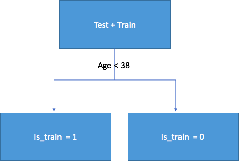
If there exist a covariate shift, then upon mixing train and test we’ll still be able to classify the origin of each data point (whether it is from test or train) with good accuracy.
Let’s understand why. Consider the above example where age was the drifting feature between test and train. If we take a classifier like Random Forest and try to classify rows into test and train, age will be come out be very important feature in splitting the data.
Implementation
Now let’s try to apply this idea on a real dataset. I’m using dataset from this kaggle competition: https://www.kaggle.com/c/porto-seguro-safe-driver-prediction/data
Step1: Data pre-processing
We have to first clean our data, impute all missing values and do label encoding for all the categorical variables. For this dataset, this step was not required so I have skipped this step.
#loading test and train data
train = pd.read_csv(‘train.csv’,low_memory=True)
test = pd.read_csv(‘test.csv’,low_memory=True)
Step2:
We have to add a feature ‘is_train’in both train and test data. Value for this feature will be 0 for test and 1 for train.
#adding a column to identify whether a row comes from train or not
test[‘is_train’] = 0
train[‘is_train’] = 1
Combining train and test
Then we have to combine both the datasets. Also since train data has the original ‘target’ variable which is not present in test, we have to drop that variable too.
Note: For your problem, ‘target’ will be replaced by the name of the dependent variable for your original problem.
#combining test and train data
df_combine = pd.concat([train, test], axis=0, ignore_index=True)
#dropping ‘target’ column as it is not present in the test
df_combine = df_combine.drop(‘target’, axis =1)
y = df_combine['is_train'].values #labels
x = df_combine.drop('is_train', axis=1).values #covariates or our independent variables
tst, trn = test.values, train.values
Step4: Building and testing a classifier
For classification purposes I’m using Random Forest Classifier to predict the labels for each row in the combined dataset. You can use any other classifier also.
m = RandomForestClassifier(n_jobs=-1, max_depth=5,min_samples_leaf = 5)
predictions = np.zeros(y.shape) #creating an empty prediction array
We are using stratified 4 fold to ensure that percentage for each class is preserved and we cover the whole data once. For each row the classifier will calculate the probability of it belonging to train.
skf = SKF(n_splits=20, shuffle=True, random_state=100)
for fold, (train_idx, test_idx) in enumerate(skf.split(x, y)):
 X_train, X_test = x[train_idx], x[test_idx]
 y_train, y_test = y[train_idx], y[test_idx]

 m.fit(X_train, y_train)
 probs = m.predict_proba(X_test)[:, 1] #calculating the probability
 predictions[test_idx] = probs
Step5: Interpreting the results
We’ll output the ROC-AUC metric for our classifier as an estimate how much covariate shift this data has.
If the classifier is able to classify the rows into train and test with good accuracy, our AUC score should be on the higher side (greater than 0.8). This implies strong covariate shift between train and test.
print(‘ROC-AUC for train and test distributions:’, AUC(y, predictions))
# ROC-AUC for train and test distributions: 0.49944573868
AUC value of 0.49 implies that there is no evidence of strong covariate shift. This means that majority of the observations comes from a feature space which is not specific to test or train.
As this dataset is taken from Kaggle, this result is quite expected. As in such kind of competition dataset is carefully curated to ensure such shifts are not there.
This process can be replicated for any data science problem to check for covariate shift before we start modeling.
Going beyond
At this point we either observe covariate shift or not. So what can we possibly do to improve our performance on the test data ??
- Dropping of drifting features
- Importance weight using Density Ratio Estimation
Dropping of drifting features:
Note: This method is applicable to the situation where you witness covariate shift.
- Extract feature importance from the random forest classifier object that we have built in the previous section
- The top features are the ones which are drifting and causing the shift
- From the top features drop one variable at a time and build your model and check its performance. Collect all the features for which performance is not degrading
- Now drop all those features while building the final model
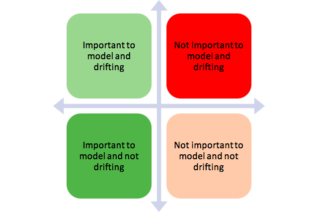
The idea is to remove the features that fall in the red bucket
Importance weight using Density Ratio Estimation
Note: This method is applicable irrespective of whether there exist a covariate shift or not.
Let’s look at the predictions that we have calculated in the previous section. For each observation, this prediction tells us the probability that it belongs to the training data according to our classifier.
predictions[:10]
----output-----
array([ 0.34593171])
So for the first row our classifier thinks that it belongs to training data with .34 probability. Let’s call this P(train). Or we can also say that it has .66 probability of being from the test data. Let’s call this as P(test). Now here is the magic trick:
For each row of training data we calculate a coefficient w = P(test)/P(train).
This w tells us how close is the observation from the training data to our test data. Here is the punchline:
We can use this w as sample weights in any of our classifier to increase the weight of these observation which seems similar to our test data. Intuitively this makes sense as our model will focus more on capturing patterns from the observations which seems similar to our test.
These weights can be calculated using the below code.
plt.figure(figsize=(20,5))
predictions_train = predictions[len(tst):] #filtering the actual training rows
weights = (1./predictions_train) — 1.
weights /= np.mean(weights) # Normalizing the weights
plt.xlabel(‘Computed sample weight’)
plt.ylabel(‘# Samples’)
sns.distplot(weights, kde=False)
< You can pass the weights calculated in the model fit method like this:
m = RandomForestClassifier(n_jobs=-1,max_depth=5)
m.fit(X_train, y_train, sample_weight=weights)
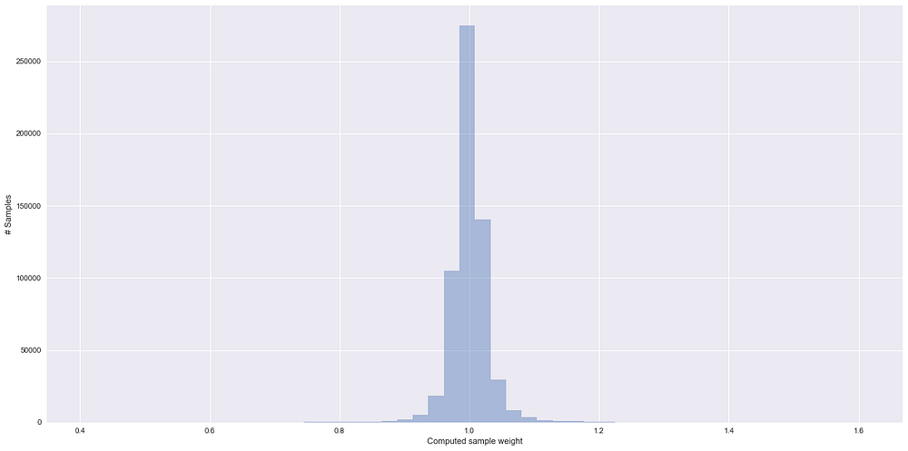
Some things to notice in the above plot:
- Higher the weight for the observation, more is it similar to the test data
- Almost 70% of training samples have sample weight of close to 1 and hence comes from a feature space which is not very specific to train or test high density region. This is in line with the AUC value that we have calculated
End Notes
I hope that now you have a better understanding about covariate shift, how you can identify it and treat it effectively.
Bio: Shikhar Gupta is pursuing masters in data science at U. of San Francisco, Intern @IsaziConsulting, alumni @iitroorkee .
Original. Reposted with permission.
Related: