Building A Data Science Product in 10 Days
At startups, you often have the chance to create products from scratch. In this article, the author will share how to quickly build valuable data science products, using his first project at Instacart as an example.
By Houtao Deng, Data scientist at Instacart.
At startups, we often have the chance to create products from scratch. In this article, I’ll share how to quickly build valuable data science products, using my first project at Instacart as an example.
Here is the problem. After adding items to the shopping cart on Instacart, a customer can select a delivery window during checkout (illustrated in Figure 1). Then, an Instacart shopper would try to deliver the groceries to the customer within the window. During peak times, our system often accepted more orders than our shoppers could handle, and some orders would be delivered late.
We decided to leverage data science to address the lateness issue. The idea was to use data science models to estimate the delivery capacity for each window, and a window would be closed when the number of orders placed reaches its capacity.
Here is how we built a v1 product in 10 days.
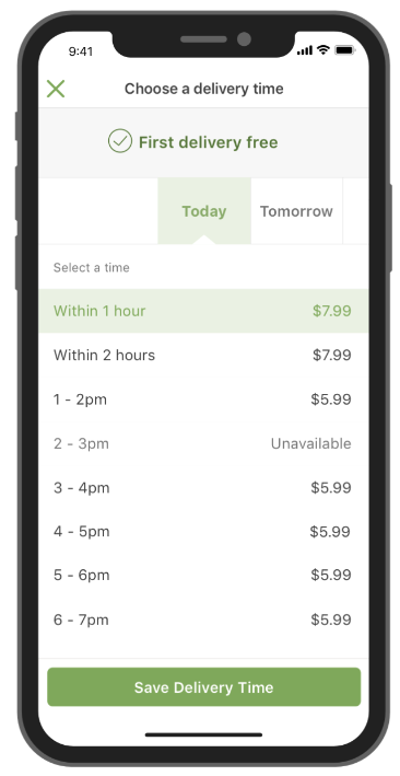
Fig 1. A customer can choose an available delivery window for the grocery items to be delivered.
Day 1. Planning
We started with planning so that we could work on the right things and develop a solution fast.
- First, we defined the metrics to measure the project progress.
- Second, we identified an area that was achievable with a high impact (low-hanging fruit).
- Third, we came up with a simple solution that could be implemented quickly.
Metrics. The percentage of late deliveries per day was used to measure lateness. We didn’t want to close delivery windows too early and fail to capture the orders that could be delivered on time. So, the number of deliveries per day was used as a counter metric. (We now use shopper utilization as a counter metric.)
Low-hanging fruit. Data showed that for days with a lot of late deliveries, the majority of the orders were placed one day before. Therefore, we decided to focus on the next-day delivery windows (Tomorrow’s windows in Figure 1).
Solution. To deliver an order within time window T (between T and T+1) , a shopper may start working on the order before T. Figure 2 illustrates that a shopper begins to work on an order in window T-2, and delivers the order in window T. As most orders took less than two hours, the capacity of a delivery window T mostly depends on the number of shoppers at time window T, T-1, and T-2.
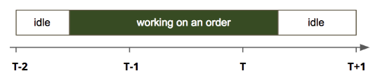
Fig 2. Illustration of a shopper’s time spent on an order.
capacity(T) = a+b0*#shoppers(T)+b1*#shoppers(T-1)+b2*#shoppers(T-2)
There can be other factors (e.g., weather) also affecting capacity, but we decided to start simple.
Day 2–3. First Iteration on Models
We followed a typical modeling process: feature engineering, creating training and testing data, and comparing different models. However, once we felt the models were reasonably accurate, we did not invest more time in models. Firstly, models were only one part of the system. Secondly, the improvement in model accuracy did not necessarily translate to the same degree of improvement in metrics.
Features and Data. For each delivery window in the past, we had the following data: the orders delivered within the window, and shoppers’ time spent on the orders. Figure 3 illustrates for three orders delivered in time window T (between T and T+1), there were 2 shoppers worked in window T-2, and 3 shoppers worked in both window T-1 and T. Figure 4 shows one row of data created from this example.
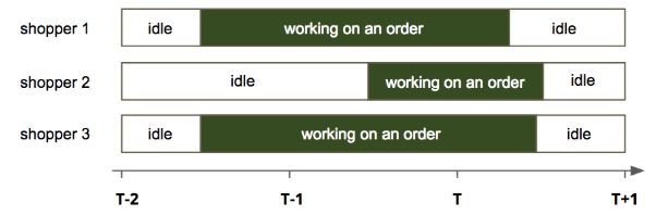
Fig 3. For the three orders delivered within time window T (between T and T+1), 2 shoppers worked in window T-2, and 3 shoppers worked in both window T-1 and T.
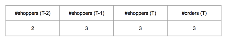
Fig 4. One row of data created from the example shown in Figure 3.
Linear model. Using #orders(T) as the response variable, other variables as the predictors, we built a linear model on a training data set and tested it on a validation data set. The form of the model is as follows
#orders(T) = a+b0*#shoppers(T)+b1*#shoppers(T-1)+b2*#shoppers(T-2)
The predicted values vs. actual values for the validation data are plotted in Figure 5 (left). The mean of the actual values at each predicted value and the 45-degree line are also plotted.
Non-linear model. We built a random forest model for comparison. The predicted values vs. actual values are plotted in Figure 5 (right). The random forest model was not substantially better than the linear model, and so we felt comfortable to proceed with the linear model that is easier to interpret and implement.
Prediction. With the linear model, we can estimate the capacity for a future delivery window T with the following formula
capacity(T) = a+b0*#shoppers(T)+b1*#shoppers(T-1)+b2*#shoppers(T-2)
Note that in this formula, #shoppers(t) represents the number of shoppers scheduled at a future time window t (t = T, T-1 or T-2).
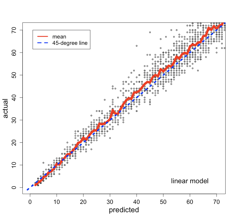
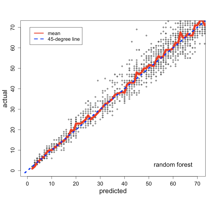
Fig 5. Predicted vs. actual plots from a linear model (left) and a random forest model (right).
Day 4–5. End-to-End Integration
We used databases as the interfaces between data science and engineering components. In this way, the dependency between data science and engineering can be reduced (vs. embedding a data science model in the engineering code), and the ownership of different components can be clearly defined. Figure 6 illustrates how the system works.
Data science components. There were two data science jobs, model training job and prediction job, both triggered by cron (a time-based scheduler) at pre-defined frequencies. The model training job ran every week, fetched the most recent order_shoppers data (orders and shoppers’ time spent on the orders), fitted the models and saved them into a database table (models). The prediction job ran every night, fetched the models and scheduled_hours (future scheduled shopper hours) data, and estimated the capacity for future delivery windows. The estimates were then saved to the capacity_estimates table.
Engineering components. The capacity counting job was created to consume capacity estimates and provide the delivery availability of each window for the customer app. It was scheduled to run every minute, got the capacity estimates and existing orders, calculated if a delivery window was available, and saved the availability information to the delivery_availabilities table. Also, when a customer placed an order, the order information would be saved to the orders table, and the capacity counting job would be triggered.
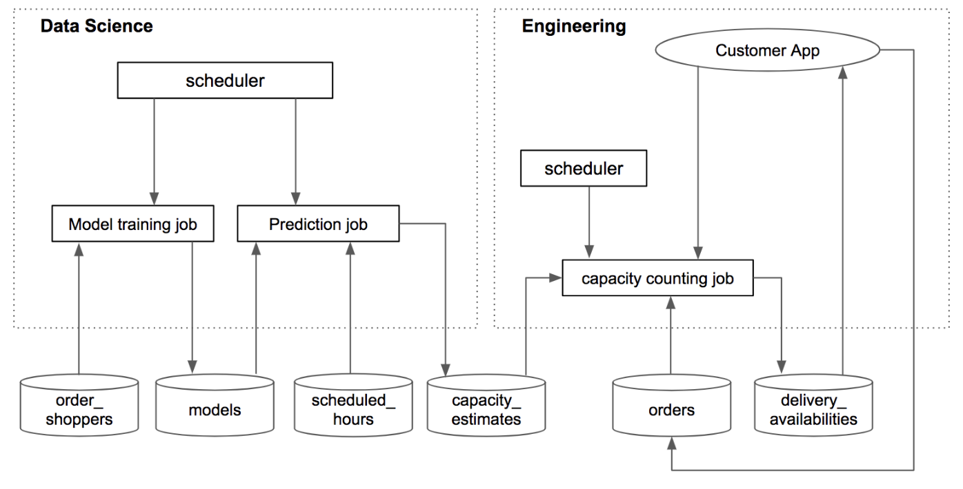
Fig 6. Integration of data science and engineering components.
Day 6–8. Second Iteration on Models
We did a sanity check on capacity estimates, and two modeling issues were found and fixed.
Sanity check. We ran the prediction job that generated the capacity estimates for future delivery windows. Then, after a window became obsolete, we compared the estimated capacity of the window to the orders actually accepted by the existing system. We found that in some cases the existing system took fewer orders than the estimated capacity but with substantial lateness (illustrated in Figure 7). This indicated the capacity was over-estimated in those cases. Based on this insight, we found two issues.
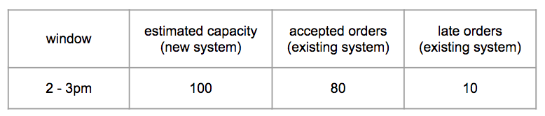
Fig 7. Validate the capacity estimates by comparing them to the orders accepted by the existing system.
Issue 1: mean prediction. The models we built predicted the mean. It can be seen from Figure 5 (left) that there are data points below the mean line. The mean predictions would over-estimate the capacity for those data points. To solve this, a prediction interval was constructed, and a lower percentile level was used. Figure 8 shows the 25th percentile and 75th percentile levels.
Issue 2: data inconsistency. #shoppers used in prediction is the number of scheduled shoppers at a future window, and shoppers can cancel their scheduled hours before the window. However, #shoppers used in model training did not include canceled hours. So, the data used for prediction and training were not consistent. To fix it, cancellation rates were estimated and included in the formula
capacity(T) = a+b0*#shoppers(T)*{1-cancelation_rate(T)}+ …

Fig 8. The 25th percentile and 75th percentile values of the actual values at each predicted value.
Day 9–10. Adjustments
Before launching the new system to customers, we started internal tests (without impacting customers) and made adjustments accordingly.
Percentile level. We adjusted the percentile level to pass the sanity check mentioned in the previous section.
Caching. Jobs were made faster by caching (storing frequently used data on the servers to avoid redundant calls to the databases).
Launch
Figure 9 shows the percentage of late deliveries by day around the product launching time. The new system achieved our goal of substantially reducing late deliveries (without reducing the number of deliveries). It was a quick success. Since the initial launch, we’ve continued to iterate, including estimating the capacity for same-day delivery windows.
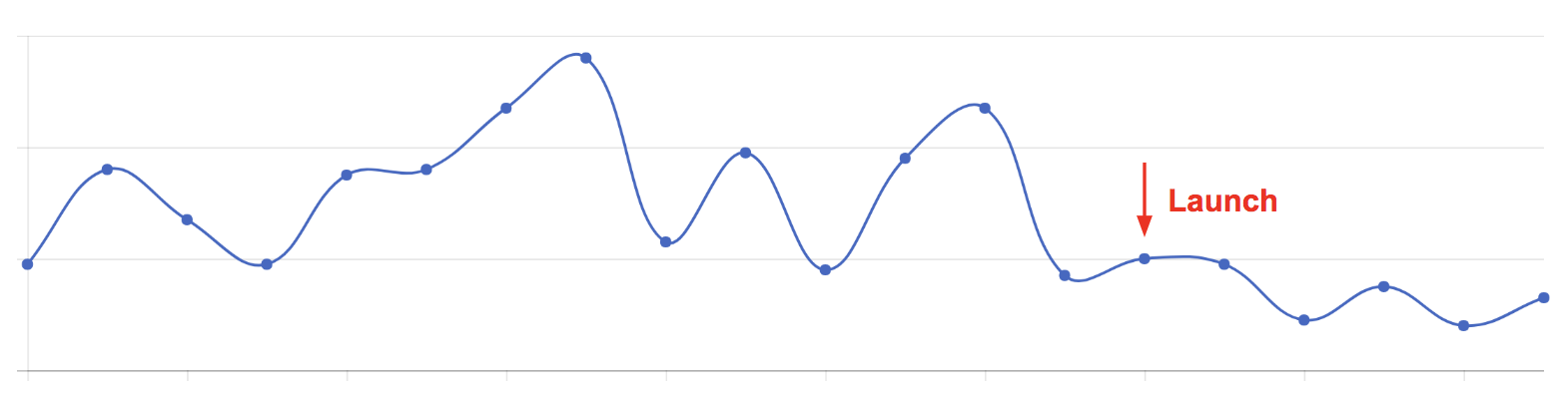
Fig 9. The percentage of late deliveries by day.
Takeaways
As a data scientist who joined a startup for the first time, I learned the following lessons in quickly building valuable data science products
- identifying impactful and achievable work
- reducing the dependency between engineering and data science components
- focusing on improving the metrics, not necessarily the model accuracy
- starting simple and iterating fast
Four years later, Instacart is now a much larger company, but the learnings are still applicable to the data science projects we do to deliver business value quickly.
Note: Andrew Kane contributed to the first version of the engineering components, and Tahir Mobashir and Sherin Kurian contributed to the later iterations.
Original. Reposted with permission.
Related: