Explaining the 68-95-99.7 rule for a Normal Distribution

comments

By Michael Galarnyk, Data Scientist

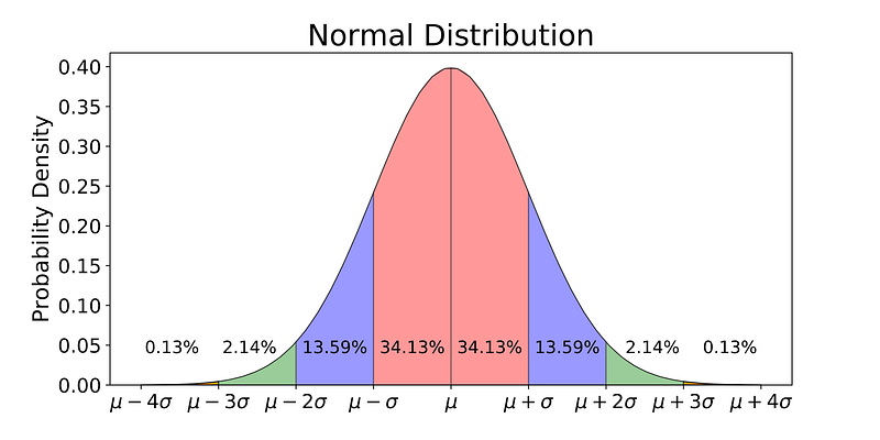
68% of the data is within 1 standard deviation, 95% is within 2 standard deviation, 99.7% is within 3 standard deviations

The normal distribution is commonly associated with the 68-95-99.7 rule which you can see in the image above. 68% of the data is within 1 standard deviation (σ) of the mean (μ), 95% of the data is within 2 standard deviations (σ) of the mean (μ), and 99.7% of the data is within 3 standard deviations (σ) of the mean (μ).

This post explains how those numbers were derived in the hope that they can be more interpretable for your future endeavors. As always, the code used to derive to make everything (including the graphs) is available on my github. With that, let’s get started!

Probability Density Function

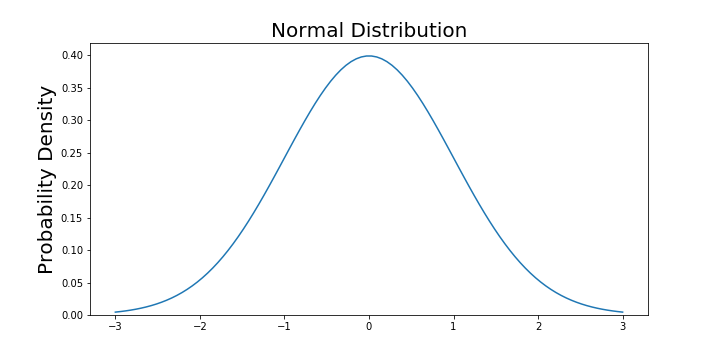
To be able to understand where the percentages come from, it is important to know about the probability density function (PDF). A PDF is used to specify the probability of the random variable falling within a particular range of values, as opposed to taking on any one value. This probability is given by the integral of this variable’s PDF over that range — that is, it is given by the area under the density function but above the horizontal axis and between the lowest and greatest values of the range. This definition might not make much sense so let’s clear it up by graphing the probability density function for a normal distribution. The equation below is the probability density function for a normal distribution

PDF for a Normal Distribution

Let’s simplify it by assuming we have a mean (μ) of 0 and a standard deviation (σ) of 1.

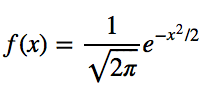
PDF for a Normal Distribution

Now that the function is simpler, let’s graph this function with a range from -3 to 3.

# Import all libraries for the rest of the blog post
from scipy.integrate import quad
import numpy as np
import matplotlib.pyplot as plt
x = np.linspace(-3, 3, num = 100)
constant = 1.0 / np.sqrt(2*np.pi)
pdf_normal_distribution = constant * np.exp((-x**2) / 2.0)
fig, ax = plt.subplots(figsize=(10, 5));
ax.plot(x, pdf_normal_distribution);
ax.set_ylim(0);
ax.set_title('Normal Distribution', size = 20);
ax.set_ylabel('Probability Density', size = 20);

The graph above does not show you the probability of events but their probability density. To get the probability of an event within a given range we will need to integrate. Suppose we are interested in finding the probability of a random data point landing within 1 standard deviation of the mean, we need to integrate from -1 to 1. This can be done with SciPy.

# Make a PDF for the normal distribution a function
def normalProbabilityDensity(x):
    constant = 1.0 / np.sqrt(2*np.pi)
    return(constant * np.exp((-x**2) / 2.0) )
# Integrate PDF from -1 to 1
result, _ = quad(normalProbabilityDensity, -1, 1, limit = 1000)
print(result)

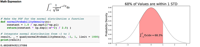
Code to integrate the PDF of a normal distribution (left) and visualization of the integral (right).

68% of the data is within 1 standard deviation (σ) of the mean (μ).

If you are interested in finding the probability of a random data point landing within 2 standard deviations of the mean, you need to integrate from -2 to 2.

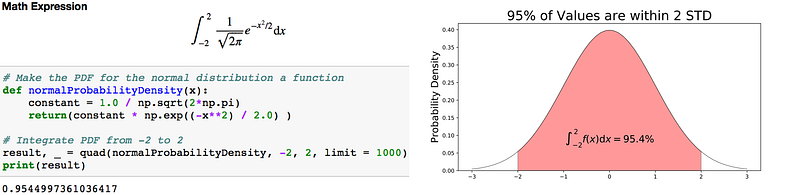
Code to integrate the PDF of a normal distribution (left) and visualization of the integral (right).

95% of the data is within 2 standard deviations (σ) of the mean (μ).

If you are interested in finding the probability of a random data point landing within 3 standard deviations of the mean, you need to integrate from -3 to 3.

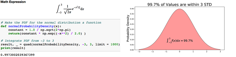
Code to integrate the PDF of a normal distribution (left) and visualization of the integral (right).

99.7% of the data is within 3 standard deviations (σ) of the mean (μ).

It is important to note that for any PDF, the area under the curve must be 1 (the probability of drawing any number from the function’s range is always 1).

You will also find that it is also possible for observations to fall 4, 5 or even more standard deviations from the mean, but this is very rare if you have a normal or nearly normal distribution.

Future tutorials will cover how to take this knowledge and apply it to box plots and confidence intervals, but that is for a later time. If you any questions or thoughts on the tutorial, feel free to reach out in the comments below or through Twitter.

 
Bio: Michael Galarnyk is a Data Scientist and Corporate Trainer. He currently works at Scripps Translational Research Institute. You can find him on Twitter (https://twitter.com/GalarnykMichael), Medium (https://medium.com/@GalarnykMichael), and GitHub (https://github.com/mGalarnyk).

Original. Reposted with permission.

Related:

• Jupyter Notebook for Beginners: A Tutorial
• Why Data Scientists Love Gaussian
• Descriptive Statistics: The Mighty Dwarf of Data Science