Topic Modeling with LSA, PLSA, LDA & lda2Vec

This article is a comprehensive overview of Topic Modeling and its associated techniques.

By Joyce Xu, Stanford

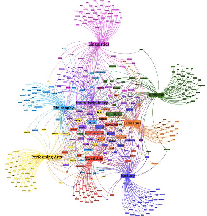
In natural language understanding (NLU) tasks, there is a hierarchy of lenses through which we can extract meaning — from words to sentences to paragraphs to documents. At the document level, one of the most useful ways to understand text is by analyzing its topics. The process of learning, recognizing, and extracting these topics across a collection of documents is called topic modeling.

In this post, we will explore topic modeling through 4 of the most popular techniques today: LSA, pLSA, LDA, and the newer, deep learning-based lda2vec.

Overview

All topic models are based on the same basic assumption:

each document consists of a mixture of topics, and
each topic consists of a collection of words.

In other words, topic models are built around the idea that the semantics of our document are actually being governed by some hidden, or “latent,” variables that we are not observing. As a result, the goal of topic modeling is to uncover these latent variables — topics — that shape the meaning of our document and corpus. The rest of this blog post will build up an understanding of how different topic models uncover these latent topics.

LSA

Latent Semantic Analysis, or LSA, is one of the foundational techniques in topic modeling. The core idea is to take a matrix of what we have — documents and terms — and decompose it into a separate document-topic matrix and a topic-term matrix.

The first step is generating our document-term matrix. Given m documents and n words in our vocabulary, we can construct an m × n matrix A in which each row represents a document and each column represents a word. In the simplest version of LSA, each entry can simply be a raw count of the number of times the j-th word appeared in the i-th document. In practice, however, raw counts do not work particularly well because they do not account for the significance of each word in the document. For example, the word “nuclear” probably informs us more about the topic(s) of a given document than the word “test.”

Consequently, LSA models typically replace raw counts in the document-term matrix with a tf-idf score. Tf-idf, or term frequency-inverse document frequency, assigns a weight for term j in document i as follows:

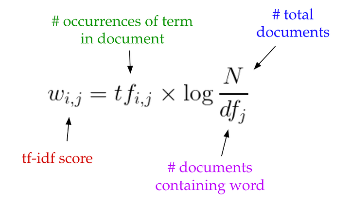
Intuitively, the more frequently the term appears in the document, the greater its weight, and the more infrequently it appears across the corpus, the greater its weight.

Once we have our document-term matrix A, we can start thinking about our latent topics. Here’s the thing: in all likelihood, A is very sparse, very noisy, and very redundant across its many dimensions. As a result, to find the few latent topics that capture the relationships among the words and documents, we want to perform dimensionality reduction on A.

This dimensionality reduction can be performed using truncated SVD. SVD, or singular value decomposition, is a technique in linear algebra that factorizes any matrix M into the product of 3 separate matrices: M=U*S*V, where S is a diagonal matrix of the singular values of M. Critically, truncated SVD reduces dimensionality by selecting only the t largest singular values, and only keeping the first t columns of U and V. In this case, t is a hyperparameter we can select and adjust to reflect the number of topics we want to find.

Intuitively, think of this as only keeping the t most significant dimensions in our transformed space.

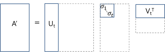
In this case, U ∈ ℝ^(m ⨉ t) emerges as our document-topic matrix, and V ∈ ℝ^(n ⨉ t) becomes our term-topic matrix. In both U and V, the columns correspond to one of our t topics. In U, rows represent document vectors expressed in terms of topics; in V, rows represent term vectors expressed in terms of topics.

With these document vectors and term vectors, we can now easily apply measures such as cosine similarity to evaluate:

the similarity of different documents
the similarity of different words
the similarity of terms (or “queries”) and documents (which becomes useful in information retrieval, when we want to retrieve passages most relevant to our search query).

Code
In sklearn, a simple implementation of LSA might look something like this:

from sklearn.feature_extraction.text import TfidfVectorizer
from sklearn.decomposition import TruncatedSVD
from sklearn.pipeline import Pipeline

documents = ["doc1.txt", "doc2.txt", "doc3.txt"] 
  
# raw documents to tf-idf matrix: 

vectorizer = TfidfVectorizer(stop_words='english', 
                             use_idf=True, 
                             smooth_idf=True)

# SVD to reduce dimensionality: 

svd_model = TruncatedSVD(n_components=100,         // num dimensions
                         algorithm='randomized',
                         n_iter=10)

# pipeline of tf-idf + SVD, fit to and applied to documents:

svd_transformer = Pipeline([('tfidf', vectorizer), 
                            ('svd', svd_model)])

svd_matrix = svd_transformer.fit_transform(documents)

# svd_matrix can later be used to compare documents, compare words, or compare queries with documents

LSA is quick and efficient to use, but it does have a few primary drawbacks:

lack of interpretable embeddings (we don’t know what the topics are, and the components may be arbitrarily positive/negative)
need for really large set of documents and vocabulary to get accurate results
less efficient representation

PLSA

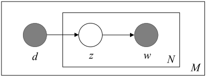
pLSA, or Probabilistic Latent Semantic Analysis, uses a probabilistic method instead of SVD to tackle the problem. The core idea is to find a probabilistic model with latent topics that can generate the data we observe in our document-term matrix. In particular, we want a model P(D,W) such that for any document d and word w, P(d,w) corresponds to that entry in the document-term matrix.

Recall the basic assumption of topic models: each document consists of a mixture of topics, and each topic consists of a collection of words. pLSA adds a probabilistic spin to these assumptions:

given a document d, topic z is present in that document with probability P(z|d)
given a topic z, word w is drawn from z with probability P(w|z)

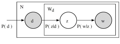
Formally, the joint probability of seeing a given document and word together is:

Intuitively, the right-hand side of this equation is telling us how likely it is see some document, and then based upon the distribution of topics of that document, how likely it is to find a certain word within that document.

In this case, P(D), P(Z|D), and P(W|Z) are the parameters of our model. P(D) can be determined directly from our corpus. P(Z|D) and P(W|Z) are modeled as multinomial distributions, and can be trained using the expectation-maximization algorithm (EM). Without going into a full mathematical treatment of the algorithm, EM is a method of finding the likeliest parameter estimates for a model which depends on unobserved, latent variables (in our case, the topics).

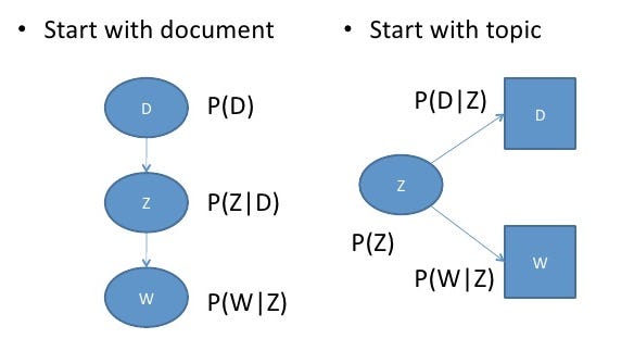
Interestingly, P(D,W) can be equivalently parameterized using a different set of 3 parameters:

We can understand this equivalency by looking at the model as a generative process. In our first parameterization, we were starting with the document with P(d), and then generating the topic with P(z|d), and then generating the word with P(w|z). In this parameterization, we are starting with the topic with P(z), and then independently generating the document with P(d|z) and the word with P(w|z).

https://www.slideshare.net/NYCPredictiveAnalytics/introduction-to-probabilistic-latent-semantic-analysis

The reason this new parameterization is so interesting is because we can see a direct parallel between our pLSA model our LSA model:

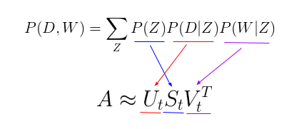
where the probability of our topic P(Z) corresponds to the diagonal matrix of our singular topic probabilities, the probability of our document given the topic P(D|Z) corresponds to our document-topic matrix U, and the probability of our word given the topic P(W|Z) corresponds to our term-topic matrix V.

So what does that tell us? Although it looks quite different and approaches the problem in a very different way, pLSA really just adds a probabilistic treatment of topics and words on top of LSA. It is a far more flexible model, but still has a few problems. In particular:

Because we have no parameters to model P(D), we don’t know how to assign probabilities to new documents
The number of parameters for pLSA grows linearly with the number of documents we have, so it is prone to overfitting

We will not look at any code for pLSA because it is rarely used on its own. In general, when people are looking for a topic model beyond the baseline performance LSA gives, they turn to LDA. LDA, the most common type of topic model, extends PLSA to address these issues.

LDA

LDA stands for Latent Dirichlet Allocation. LDA is a Bayesian version of pLSA. In particular, it uses dirichlet priors for the document-topic and word-topic distributions, lending itself to better generalization.

I am not going to into an in-depth treatment of dirichlet distributions, since there are very good intuitive explanations here and here. As a brief overview, however, we can think of dirichlet as a “distribution over distributions.” In essence, it answers the question: “given this type of distribution, what are some actual probability distributions I am likely to see?”

Consider the very relevant example of comparing probability distributions of topic mixtures. Let’s say the corpus we are looking at has documents from 3 very different subject areas. If we want to model this, the type of distribution we want will be one that very heavily weights one specific topic, and doesn’t give much weight to the rest at all. If we have 3 topics, then some specific probability distributions we’d likely see are:

Mixture X: 90% topic A, 5% topic B, 5% topic C
Mixture Y: 5% topic A, 90% topic B, 5% topic C
Mixture Z: 5% topic A, 5% topic B, 90% topic C

If we draw a random probability distribution from this dirichlet distribution, parameterized by large weights on a single topic, we would likely get a distribution that strongly resembles either mixture X, mixture Y, or mixture Z. It would be very unlikely for us to sample a distribution that is 33% topic A, 33% topic B, and 33% topic C.

That’s essentially what a dirichlet distribution provides: a way of sampling probability distributions of a specific type. Recall the model for pLSA:

In pLSA, we sample a document, then a topic based on that document, then a word based on that topic. Here is the model for LDA:

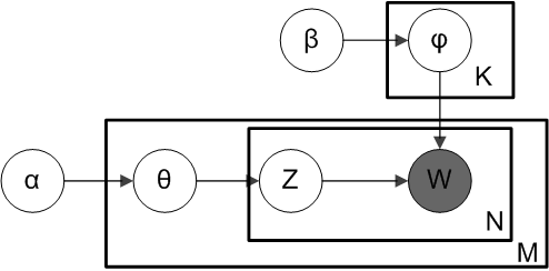
From a dirichlet distribution Dir(α), we draw a random sample representing the topic distribution, or topic mixture, of a particular document. This topic distribution is θ. From θ, we select a particular topic Z based on the distribution.

Next, from another dirichlet distribution Dir(????), we select a random sample representing the word distribution of the topic Z. This word distribution is φ. From φ, we choose the word w.

Formally, the process for generating each word from a document is as follows (beware this algorithm uses c instead of z to represent the topic):

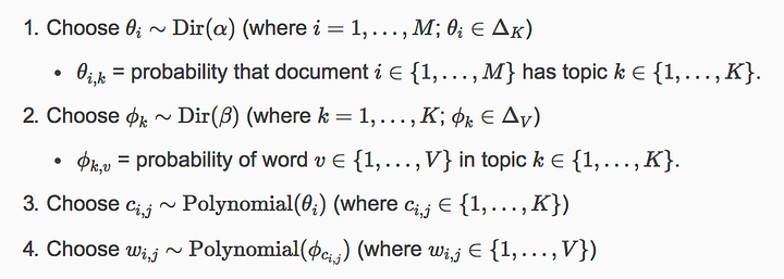
https://cs.stanford.edu/~ppasupat/a9online/1140.html

LDA typically works better than pLSA because it can generalize to new documents easily. In pLSA, the document probability is a fixed point in the dataset. If we haven’t seen a document, we don’t have that data point. In LDA, the dataset serves as training data for the dirichlet distribution of document-topic distributions. If we haven’t seen a document, we can easily sample from the dirichlet distribution and move forward from there.

Code

LDA is easily the most popular (and typically most effective) topic modeling technique out there. It’s available in gensim for easy use:

from gensim.corpora.Dictionary import load_from_text, doc2bow
from gensim.corpora import MmCorpus
from gensim.models.ldamodel import LdaModel

document = "This is some document..."

# load id->word mapping (the dictionary)
id2word = load_from_text('wiki_en_wordids.txt')

# load corpus iterator
mm = MmCorpus('wiki_en_tfidf.mm')

# extract 100 LDA topics, updating once every 10,000
lda = LdaModel(corpus=mm, id2word=id2word, num_topics=100, update_every=1, chunksize=10000, passes=1)

# use LDA model: transform new doc to bag-of-words, then apply lda
doc_bow = doc2bow(document.split())
doc_lda = lda[doc_bow]

# doc_lda is vector of length num_topics representing weighted presence of each topic in the doc

With LDA, we can extract human-interpretable topics from a document corpus, where each topic is characterized by the words they are most strongly associated with. For example, topic 2 could be characterized by terms such as “oil, gas, drilling, pipes, Keystone, energy,” etc. Furthermore, given a new document, we can obtain a vector representing its topic mixture, e.g. 5% topic 1, 70% topic 2, 10% topic 3, etc. These vectors are often very useful for downstream applications.

LDA in Deep Learning: lda2vec

So where do these topic models factor in to more complex natural language processing problems?

At the beginning of this post, we talked about how important it is to be able to extract meaning from text at every level — word, paragraph, document. At the document level, we now know how to represent the text as mixtures of topics. At the word level, we typically use something like word2vec to obtain vector representations. lda2vec is an extension of word2vec and LDA that jointly learns word, document, and topic vectors.

Here’s how it works.

lda2vec specifically builds on top of the skip-gram model of word2vec to generate word vectors. If you’re not familiar with skip-gram and word2vec, you can read up on it here, but essentially it’s a neural net that learns a word embedding by trying to use the input word to predict surrounding context words.

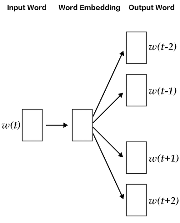
With lda2vec, instead of using the word vector directly to predict context words, we leverage a context vector to make the predictions. This context vector is created as the sum of two other vectors: the word vector and the document vector.

The word vector is generated by the same skip-gram word2vec model discussed earlier. The document vector is more interesting. It is really a weighted combination of two other components:

the document weight vector, representing the “weights” (later to be transformed into percentages) of each topic in the document
the topic matrix, representing each topic and its corresponding vector embedding

Together, the document vector and the word vector generate “context” vectors for each word in the document. The power of lda2vec lies in the fact that it not only learns word embeddings (and context vector embeddings) for words, it simultaneously learns topic representations and document representations as well.

https://multithreaded.stitchfix.com/blog/2016/05/27/lda2vec

For a more detailed overview of the model, check out Chris Moody’s original blog post (Moody created lda2vec in 2016). Code can be found at Moody’s github repository and this Jupyter Notebook example.

Conclusion

All too often, we treat topic models as black-box algorithms that “just work.” Fortunately, unlike many neural nets, topic models are actually quite interpretable and much more straightforward to diagnose, tune, and evaluate. Hopefully this blog post has been able to explain the underlying math, motivations, and intuition you need, and leave you enough high-level code to get started. Please leave your thoughts in the comments, and happy hacking!

This is part of a series created for Nanonets.

Nanonets makes it super easy to use Deep Learning.

You can build a model with your own data to achieve high accuracy & use our APIs to integrate the same in your application.

For further details visit us here or reach out to us at info@nanonets.com

Bio: Joyce Xu is a self-taught artificial intelligence and machine learning engineer. Over the past two years, she has worked on everything from AI-powered education technology products in Silicon Valley to real-time computer vision applications in satellite imagery. She is currently studying at Stanford University.

Original. Reposted with permission.

Related: