An Intuitive Guide to Deep Network Architectures
How and why do different Deep Learning models work? We provide an intuitive explanation for 3 very popular DL models: Resnet, Inception, and Xception.
By Joyce Xu, Stanford.

Over the past few years, much of the progress in deep learning for computer vision can be boiled down to just a handful of neural network architectures. Setting aside all the math, the code, and the implementation details, I wanted to explore one simple question: how and why do these models work?
At the time of writing, Keras ships with six of these pre-trained models already built into the library:
- VGG16
- VGG19
- ResNet50
- Inception v3
- Xception
- MobileNet
The VGG networks, along with the earlier AlexNet from 2012, follow the now archetypal layout of basic conv nets: a series of convolutional, max-pooling, and activation layers before some fully-connected classification layers at the end. MobileNet is essentially a streamlined version of the Xception architecture optimized for mobile applications. The remaining three, however, truly redefine the way we look at neural networks.
This rest of this post will focus on the intuition behind the ResNet, Inception, and Xception architectures, and why they have become building blocks for so many subsequent works in computer vision.
ResNet
ResNet was born from a beautifully simple observation: why do very deep nets perform worse as you keep adding layers?
Intuitively, deeper nets should perform no worse than their shallower counterparts, at least at train time (when there is no risk of overfitting). As a thought experiment, let’s say we’ve built a net with n layers that achieves a certain accuracy. At minimum, a net with n+1 layers should be able to achieve the exact same accuracy, if only by copying over the same first nlayers and performing an identity mapping for the last layer. Similarly, nets of n+2, n+3, and n+4 layers could all continue performing identity mappings and achieve the same accuracy. In practice, however, these deeper nets almost always degrade in performance.
The authors of ResNet boiled these problems down to a single hypothesis: direct mappings are hard to learn. And they proposed a fix: instead of trying to learn an underlying mapping from x to H(x), learn the difference between the two, or the “residual.” Then, to calculate H(x), we can just add the residual to the input.
Say the residual is F(x)=H(x)-x. Now, instead of trying to learn H(x) directly, our nets are trying to learn F(x)+x.
This gives rise to the famous ResNet (or “residual network”) block you’ve probably seen:
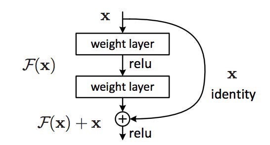
Each “block” in ResNet consists of a series of layers and a “shortcut” connection adding the input of the block to its output. The “add” operation is performed element-wise, and if the input and output are of different sizes, zero-padding or projections (via 1×1 convolutions) can be used to create matching dimensions.
If we go back to our thought experiment, this simplifies our construction of identity layers greatly. Intuitively, it’s much easier to learn to push F(x) to 0 and leave the output as x than to learn an identity transformation from scratch. In general, ResNet gives layers a “reference” point — x — to start learning from.
This idea works astoundingly well in practice. Previously, deep neural nets often suffered from the problem of vanishing gradients, in which gradient signals from the error function decreased exponentially as they backpropogated to earlier layers. In essence, by the time the error signals traveled all the way back to the early layers, they were so small that the net couldn’t learn. However, because the gradient signal in ResNets could travel back directly to early layers via shortcut connections, we could suddenly build 50-layer, 101-layer, 152-layer, and even (apparently) 1000+ layer nets that still performed well. At the time, this was a huge leap forward from the previous state-of-the-art, which won the ILSVRC 2014 challenge with 22 layers.
ResNet is one of my personal favorite developments in the neural network world. So many deep learning papers come out with minor improvements from hacking away at the math, the optimizations, and the training process without thought to the underlying task of the model. ResNet fundamentally changed the way we understand neural networks and how they learn.
Fun facts:
- The 1000+ layer net is open-source! I would not really recommend you try re-training it, but…
- If you’re feeling functional and a little frisky, I recently ported ResNet50 to the open-source Clojure ML library Cortex. Try it out and see how it compares to Keras!
Inception
If ResNet was all about going deeper, the Inception Family™ is all about going wider. In particular, the authors of Inception were interested in the computational efficiency of training larger nets. In other words: how can we scale up neural nets without increasing computational cost?
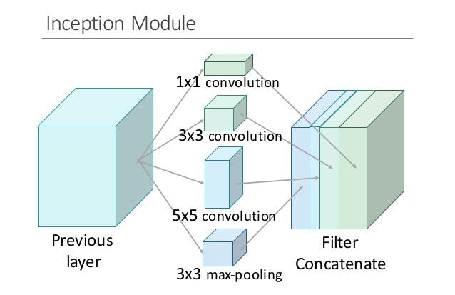
The original paper focused on a new building block for deep nets, a block now known as the “Inception module.” At its core, this module is the product of two key insights.
The first insight relates to layer operations. In a traditional conv net, each layer extracts information from the previous layer in order to transform the input data into a more useful representation. However, each layer type extracts a different kind of information. The output of a 5×5 convolutional kernel tells us something different from the output of a 3×3 convolutional kernel, which tells us something different from the output of a max-pooling kernel, and so on and so on. At any given layer, how do we know what transformation provides the most “useful” information?
Insight #1: why not let the model choose?
An Inception module computes multiple different transformations over the same input map in parallel, concatenating their results into a single output. In other words, for each layer, Inception does a 5×5 convolutional transformation, and a 3×3, and a max-pool. And the next layer of the model gets to decide if (and how) to use each piece of information.
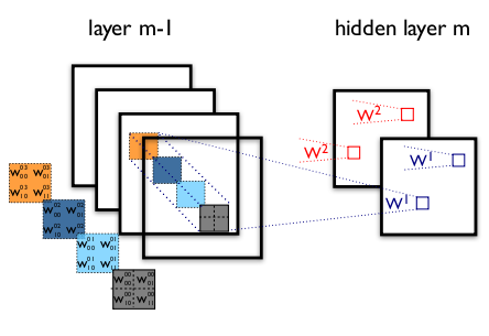
The increased information density of this model architecture comes with one glaring problem: we’ve drastically increased computational costs. Not only are large (e.g. 5×5) convolutional filters inherently expensive to compute, stacking multiple different filters side by side greatly increases the number of feature maps per layer. And this increase becomes a deadly bottleneck in our model.
Think about it this way. For each additional filter added, we have to convolve over all the input maps to calculate a single output. See the image below: creating one output map from a single filter involves computing over every single map from the previous layer.