Word Morphing – an original idea
In this post, we describe how to utilise word2vec's embeddings and A* search algorithm to morph between words.

Smooth image transition (morphing) from a tiger to a human (image courtesy: Google Images)
In order to perform word morphing, we’ll define a graph G where the set of nodes N represent words, and there’s some non negative weight function f:N×N→ℝ. Given a start word S and an end word E, our goal is to find a path within the graph which minimizes the sum of weights induced by f:

Fig. 1. Optimal path with minimal cost induced by f
Usually when people talk about word morphing they mean searching for a path between S and E where there’s an edge only between words such that one can be achieved from the other by changing one letter, as can be seen here. In this case, f(n₁,n₂) is 1 when such a change exists, and ∞ otherwise.
In this post I’ll show you how to morph between semantically similar words, i.e. f will be related to semantics. Here’s an example to illustrate the difference between the two approaches: given S=tooth, E=light, the approach of changing one character at a time can result in
tooth, booth, boots, botts, bitts, bitos, bigos, bigot, bight, light
while the semantics approach which will be defined in this post results in
tooth, retina, X_ray, light
You can find the entire code here.
Word Semantics
In order to capture word semantics we’ll use pre-trained word2vec embeddings [1]. To those of you who are not familiar with the algorithm, here’s an excerpt from Wikipedia:
Word2vec takes as its input a large corpus of text and produces a vector space, typically of several hundred dimensions, with each unique word in the corpus being assigned a corresponding vector in the space. Word vectors are positioned in the vector space such that words that share common contexts in the corpus are located in close proximity to one another in the space.
It means every node in the graph can be associated with some vector in high dimensionality space (300 in our case). Therefore, we can naturally define a distance function between every two nodes. We’ll use cosine similarity, since this is the metric usually used when one wants to semantically compare between word embeddings. From now on, I’ll overload a node symbol n to be its associated word’s embedding vector.
To use the word2vec embeddings, we’ll download Google’s pre-trained embeddings from here, and use gensim package to access them.
Choosing the Weight Function
Given the cosine similarity distance function, we can define our f function to be
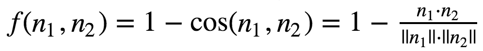
Eq. 1. Definition of weight function using cosine similarity
However, using this approach we’ll face a problem: the best path might include edges with high weight, which will result in successive words that aren’t semantically similar.
To tackle this, we can change f to be
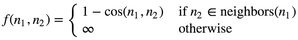
Eq. 2. Definition of weight function using cosine similarity limited to nearest neighbors
where neighbors(n₁) denotes the nearest nodes in the graph to n₁ in terms of cosine similarity. The number of neighbors is configurable.
A* Search
Now that we have our graph defined, we’ll use a well known search algorithm called A* [2].
In this algorithm, every node has a cost composed of two terms - g(n)+h(n).
g(n) is the cost of the shortest path from S to n, and h(n) is a heuristic estimating the cost of the shortest path from n to E. In our case, the heuristic function will be f.
The search algorithm maintains a data structure called the open set. Initially this set contains S, and at each iteration of the algorithm we pop out the node in the open set with the minimal cost g(n)+h(n), and add its neighbors to the open set. The algorithm stops when the node with the minimal cost is E.
This algorithm works with whatever heuristic function we choose. But in order to actually find the optimal path, the heuristic function must be admissible, meaning it can’t overestimate the true cost. Unfortunately, f is not admissible. However, we’ll use the observation that if the vectors have length 1, then the cosine similarity can be obtained using a monotonic transformation over the euclidean distance. It means the two are interchangeable in terms of ranking words by similarity. The euclidean distance is admissible (you can prove it using the triangle inequality), so we can use that instead, by defining
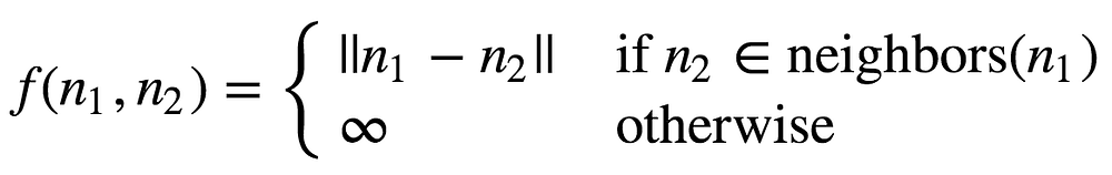
Eq. 3. Definition of weight function using euclidean distance
So to sum up, we’ll normalize the word embeddings, use the euclidean distance as a mean to find semantically similar words, and the same euclidean distance to direct A* search process in order to find the optimal path.
I chose neighbors(n) to include its 1000 nearest nodes. However, in order to make the search more efficient, we can dilute these using dilute_factor of 10: we pick the nearest neighbor, the 10'th nearest neighbor, the 20'th, and so on - until we have 100 nodes. The intuition behind it is that the best path from some intermediate node to E might pass through its nearest neighbor. If it doesn't, it might be the case that it won't pass through the second neighbor neither, since the first and second neighbors might be almost the same. So to save some computations, we just skip some of the nearest neighbors.
And here comes the fun part:
The results:
['tooth', u'retina', u'X_ray', u'light']
['John', u'George', u'Frank_Sinatra', u'Wonderful', u'perfect']
['pillow', u'plastic_bag', u'pickup_truck', u'car']
Final thoughts
Implementing the word morphing project was fun, but not as fun as playing around and trying this tool on whatever pair of words I could have thought of. I encourage you to go ahead and play with it yourself. Let me know in the comments what interesting and surprising morphings you have found :)
This post was originally posted at www.anotherdatum.com.
References
[1] https://papers.nips.cc/paper/5021-distributed-representations-of-words-and-phrases-and-their-compositionality
[2] https://www.cs.auckland.ac.nz/courses/compsci709s2c/resources/Mike.d/astarNilsson.pdf
Bio: Yoel Zeldes is a Algorithms Engineer at Taboola and is also a Machine Learning enthusiast, who especially enjoys the insights of Deep Learning.
Original. Reposted with permission.
Resources:
- on-line and web-based: Analytics, Data Mining, Data Science, Machine Learning education
- Software for Analytics, Data Science, Data Mining, and Machine Learning
Related: