 Introduction to Statistics for Data Science
 Introduction to Statistics for Data Science
This tutorial helps explain the central limit theorem, covering populations and samples, sampling distribution, intuition, and contains a useful video so you can continue your learning.
Although the Central Limit Theorem can be set as part of the “Advanced Level — The Fundamentals of Inferential Statistics with Probability Distributions” post, it is my belief this theorem deserves a single post!
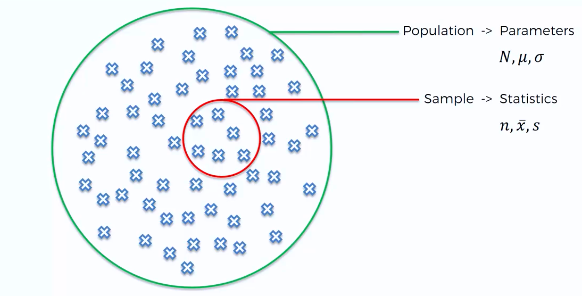
The first step of every statistical analysis you will perform is to determine whether the dataset you are dealing with is a population or a sample. As you might recall, a population is a collection of all items of interest in your study whereas a sample is a subset of data points from that population. Let’s take a short refresher!
Populations and Samples
- Population : it’s a number of something we are observing, humans, events, animals etc. It has some parameters such as the mean, median, mode, standard deviation, among others.
- Sample: it is a random subset from the population. Usually you use samples when the population is big enough to difficult the analysis of the whole set. In a sample you don’t have parameters you have statistics.
SuperDataScience Statistics For Business Analytics A-Z
Central Limit Theorem
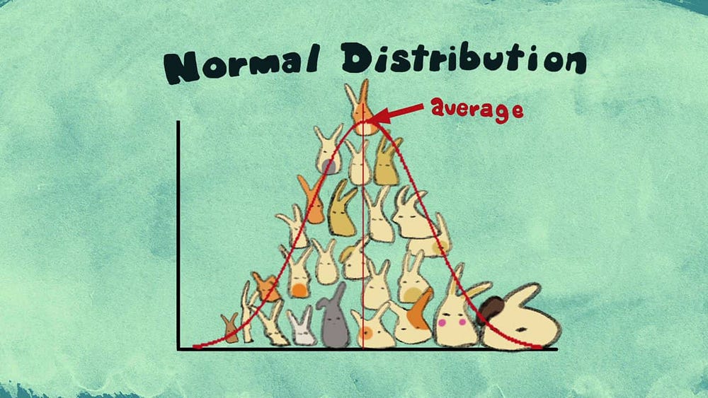
It is said to be the most important theorem of Statistics as well as Mathematics. It can be very powerful when assessing problems and world situations! The Central Limit Theorem states that
the sampling distribution will look like a normal distribution regardless of the population you are analyzing.
Sampling Distribution
As we’ve seen you take a sample to estimate the parameters of the whole population. However, not always only by sampling are you to retrieve the correct estimate of the population’s real parameters.
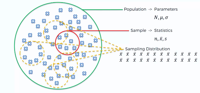
Instead of taking a single sample, what about if we take several samples from our population? For each sample, we’ll calculate the mean. So, in the end, we’ll have several values of mean estimation and then we can plot them on a chart.
SuperDataScience Statistics For Business Analytics A-Z
This will be called the sampling distribution of the sample mean.
Central Limit Theorem — Intuition
Let’s learn by looking at an example. Imagine we wanted to see the distribution of the heights in every male in the Portuguese population.
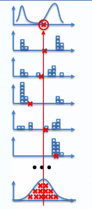
First we take several samples (heights of different man) from our population and for each sample group we calculate the respective mean. For example, we can have groups where the height is 176 cm, others with 182cm, others with 172cm, and so on. We then plot this sample mean distribution. The following picture depicts the distribution of our several samples with the x mark, in each, referring to the mean value.
SuperDataScience Statistics For Business Analytics A-Z
You can see that although you sampling means (red X marks) might be on the extremes of the general distribution most of them tend to be closer to the center.
In the end, the distribution of all these samples’ mean will present a normal distribution. Take a look at the last chart which is composed of the distribution of all the samples’ mean.
For only 5 samples you can already see that most of the means tend to concentrate towards the center of the sampling distribution. And amazingly, in the end, the mean of the sampling distribution will match the mean of the original distribution of the population.
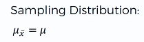
So there are two certainties with the Central Limit Theorem:
- The sampling distribution will always be normal or close to normal;
- The mean of sampling distribution will be equal to the population’s mean distribution;

- The standard error of your sampling distribution is directly linked to the standard deviation of the original population. nis equal to the number of values you take for each sample.

Let’s look at a more visual example with this GIF. The population already showed a normal distribution but later you can try with other shapes and even draw your own. We start by taking samples of size n=5 from the population and calculating the respective mean. As you increase the number of samples with n= 5 you see that the distribution of the means starts to be shaped like a normal distribution. When we increase the process several times in the thousands we get a normal distribution with a mean equal to the population’s mean. The more samples you get the more narrower the Normal distribution will be.
Now you try it! You can literally draw your distribution on this website using your mouse. Like the one you see here.
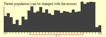
So if we start taking samples and calculating the mean of each one of those samples then plot them in a sampling distribution then you’ll obtain a normal distribution centered on the initial mean.
Access it here:
http://onlinestatbook.com/stat_sim/sampling_dist/index.html
For more content on Central Limit Theorem see this great video by CreatureCast!
CreatureCast - Central Limit Theorem from Casey Dunn on Vimeo.
Bio: Diogo Menezes Borges is a Data Scientist with a background in engineering and 2 years of experience using predictive modeling, data processing, and data mining algorithms to solve challenging business problems.
Original. Reposted with permission.
Resources:
- On-line and web-based: Analytics, Data Mining, Data Science, Machine Learning education
- Software for Analytics, Data Science, Data Mining, and Machine Learning
Related: