Artificial Neural Network Implementation using NumPy and Image Classification

comments

This tutorial builds artificial neural network in Python using NumPy from scratch in order to do an image classification application for the Fruits360 dataset. Everything (i.e. images and source codes) used in this tutorial, rather than the color Fruits360 images, are exclusive rights for my book cited as "Ahmed Fawzy Gad 'Practical Computer Vision Applications Using Deep Learning with CNNs'. Dec. 2018, Apress, 978-1-4842-4167-7 ". The book is available at Springer at this link: https://springer.com/us/book/9781484241660 .

The source code used in this tutorial is available in my GitHub page here: https://github.com/ahmedfgad/NumPyANN

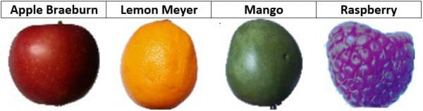
The example being used in the book is about classification of the Fruits360 image dataset using artificial neural network (ANN). The example does not assume that the reader neither extracted the features nor implemented the ANN as it discusses what the suitable set of features for use are and also how to implement the ANN in NumPy from scratch. The Fruits360 dataset has 60 classes of fruits such as apple, guava, avocado, banana, cherry, dates, kiwi, peach, and more. For making things simpler, it just works on 4 selected classes which are apple Braeburn, lemon Meyer, mango, and raspberry. Each class has around 491 images for training and another 162 for testing. The image size is 100x100 pixels.

Feature Extraction

 
The book starts by selecting the suitable set of features in order to achieve the highest classification accuracy. Based on the sample images from the 4 selected classes shown below, it seems that their color is different. This is why the color features are suitable ones for use in this task.

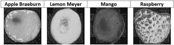
The RGB color space does not isolates color information from other types of information such as illumination. Thus, if the RGB is used for representing the images, the 3 channels will be involved in the calculations. For such a reason, it is better to use a color space that isolates the color information into a single channel such as HSV. The color channel in this case is the hue channel (H). The next figure shows the hue channel of the 4 samples presented previously. We can notice how the hue value for each image is different from the other images.

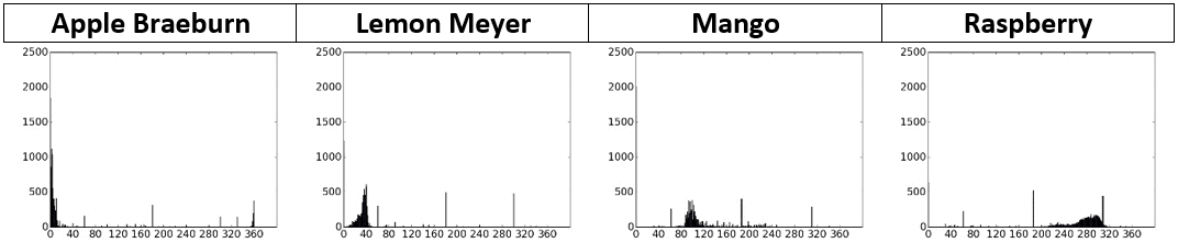
The hue channel size is still 100x100. If the entire channel is applied to the ANN, then the input layer will have 10,000 neurons. The network is still huge. In order to reduce the amounts of data being used, we can use the histogram for representing the hue channel. The histogram will have 360 bins reflecting the number of possible values for the hue value. Here are the histograms for the 4 sample images. Using a 360 bins histogram for the hue channel, it seems that every fruit votes to some specific bins of the histogram. There is less overlap among the different classes compared to using any channel from the RGB color space. For example, the bins in the apple histogram range from 0 to 10 compared to mango with its bins range from 90 to 110. The margin between each of the classes makes it easier to reduce the ambiguity in classification and thus increasing the prediction accuracy.

Here is the code that calculates the hue channel histogram from the 4 images.

import numpy
import skimage.io, skimage.color
import matplotlib.pyplot

raspberry = skimage.io.imread(fname="raspberry.jpg", as_grey=False)
apple = skimage.io.imread(fname="apple.jpg", as_grey=False)
mango = skimage.io.imread(fname="mango.jpg", as_grey=False)
lemon = skimage.io.imread(fname="lemon.jpg", as_grey=False)

apple_hsv = skimage.color.rgb2hsv(rgb=apple)
mango_hsv = skimage.color.rgb2hsv(rgb=mango)
raspberry_hsv = skimage.color.rgb2hsv(rgb=raspberry)
lemon_hsv = skimage.color.rgb2hsv(rgb=lemon)

fruits = ["apple", "raspberry", "mango", "lemon"]
hsv_fruits_data = [apple_hsv, raspberry_hsv, mango_hsv, lemon_hsv]
idx = 0
for hsv_fruit_data in hsv_fruits_data:
fruit = fruits[idx]
hist = numpy.histogram(a=hsv_fruit_data[:, :, 0], bins=360)
matplotlib.pyplot.bar(left=numpy.arange(360), height=hist[0])
matplotlib.pyplot.savefig(fruit+"-hue-histogram.jpg", bbox_inches="tight")
matplotlib.pyplot.close("all")
idx = idx + 1

By looping through all images in the 4 image classes used, we can extract the features from all images. The next code does this. According to the number of images in the 4 classes (1,962) and the feature vector length extracted from each image (360), a NumPy array of zeros is created and saved in the dataset_features variable. In order to store the class label for each image, another NumPy array named outputs is created. The class label for apple is 0, lemon is 1, mango is 2, and raspberry is 3. The code expects that it runs in a root directory in which there are 4 folders named according to the fruits names listed in the list named fruits. It loops through all images in all folders, extract the hue histogram from each of them, assign each image a class label, and finally saves the extracted features and the class labels using the pickle library. You can also use NumPy for saving the resultant NumPy arrays rather than pickle.

import numpy
import skimage.io, skimage.color, skimage.feature
import os
import pickle

fruits = ["apple", "raspberry", "mango", "lemon"]
#492+490+490+490=1,962

dataset_features = numpy.zeros(shape=(1962, 360))
outputs = numpy.zeros(shape=(1962))
idx = 0
class_label = 0

for fruit_dir in fruits:
  curr_dir = os.path.join(os.path.sep, fruit_dir)
  all_imgs = os.listdir(os.getcwd()+curr_dir)
  for img_file in all_imgs:
    fruit_data = skimage.io.imread(fname=os.getcwd()+curr_dir+img_file, as_grey=False)
    fruit_data_hsv = skimage.color.rgb2hsv(rgb=fruit_data)
    hist = numpy.histogram(a=fruit_data_hsv[:, :, 0], bins=360)
    dataset_features[idx, :] = hist[0]
    outputs[idx] = class_label
    idx = idx + 1
  class_label = class_label + 1

with open("dataset_features.pkl", "wb") as f:
  pickle.dump("dataset_features.pkl", f)

with open("outputs.pkl", "wb") as f:
  pickle.dump(outputs, f)

Currently, each image is represented using a feature vector of 360 elements. Such elements are filtered in order to just keep the most relevant elements for differentiating the 4 classes. The reduced feature vector length is 102 rather than 360. Using less elements helps to do faster training than before. The dataset_features variable shape will be 1962x102. You can read more in the book for reducing the feature vector length.

Up to this point, the training data (features and class labels) are ready. Next is implement the ANN using NumPy.