What Does a Lady Tasting Tea Have to Do with Science?
Design of Experiments (DOE) is a statistical concept used to find the cause-and-effect relationships. Surprisingly, an experiment arising from a casual conversation about tea-drinking is one of the first examples of an experiment designed using statistical ideas.
By Shane Pederson, Open Data Group.
The statistical Design of Experiments (DOE) is one of the foundational components of scientific inquiry. It enables researchers to test competing theories of how the world works, and provides a framework for evaluating the weight of evidence from a study. Less than a century old, DOE has made possible scientific advances and is a standard part of not only scientific experiments but experiments conducted out in the world: surveys, marketing studies, credit decisions are all conducted (or should be) using basic experimental design principles.

Yet not many people know that a experiment arising from a casual conversation at an English university about tea-drinking is one of the first examples of an experiment designed using statistical ideas, by a geneticist named Ronald Aylmer (R.A.) Fisher.
The Lady Tasting Tea
By the 1900’s, scientific experiments had been conducted for hundreds of years. However, results were often a mish-mash of conflicting information and sloppy procedures. The experiments themselves were rarely described, but the conclusions were stated as if fact. Fisher had been working since the turn of the century on various agricultural experiments, and had been thinking about ways in which the conduct of an experiment was itself a source of scientific inquiry. As these ideas coalesced, one summer afternoon in the 1920’s at Cambridge University, several colleagues were having a conversation when Fisher offered a phycologist, Muriel Bristol, a cup of tea. She declined after watching Fisher prepare it, saying that she preferred the taste when the milk was poured in the cup first. Fisher and others scoffed at this and a colleague, William Roach, suggested a test.
Fisher then quickly constructed a test, presenting Ms. Bristol with 8 cups of tea, 4 of which had milk poured in first, and 4 of which had milked added after the tea, but which otherwise were the same in terms of appearance, temperature, etc. They then asked her to taste all 8 and to identify the ones that had milk poured in first. The “test,” as it were, was to determine if Ms. Bristol had any ability to discern the order in which tea and milk were poured in a cup.
How would such a test work? Even if the lady had no ability to distinguish milk-first from tea-first, she would be expected to get a couple of the milk-first cups by chance. Fisher’s insight was to quantify the relative likelihood of the experimental outcome, given the lady had no ability. In essence, this was the null hypothesis  that the experiment was designed to collect evidence about.
Ms. Bristol was to choose 4 cups out of 8 as milk-first. Using a little bit of combinatorics, it turns out that there are = 70 distinct ways of choosing 4 out of 8 without regard to order. (To see this, note that there are 8* 7 * 6 * 5 = 1680 ways of choosing 4 out of 8 but 4 * 3 * 2 *1 = 24 different ways of ordering each set of 4, so we get 1680/24 = 70 ways of selecting 4 out of 8 without regard to order). With no ability to distinguish between cups, and no ability to distinguish milk-first, each of the 70 possible selections by the lady is equally likely.
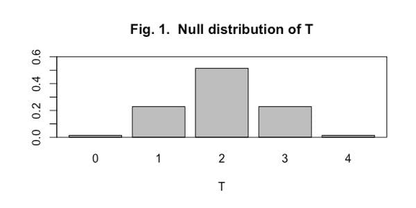
Implicit here is the concept of a test statistic T, the quantity that the test is designed to observe. T in this case is the number of cups the lady correctly selects as being milk-first, and can take on integer values between 0 (all wrong) and 4 (all right). Under the null hypothesis of no ability, one can compute the likelihood of observing each potential outcome of T:
- Where x is the number of correct choices. (This is an example of a hypergeometric distribution; more on that a bit later.)
- The probability of observing a perfect prediction, 4 out of 4, and the chance of getting three out of four is correct.
That is, if Ms. Bristol had no ability, a result as extreme as 4 correct choices would be expected 1.4% of the time, which is quite rare and evidence against the null hypothesis. 3 out of 4 would occur nearly 1/4 of the time (17/70 = 0.243), a much less rare result under H0.
The actual outcome of the experiment has always been under some dispute, although many believe that Ms. Bristol did indeed correctly identify all four milk-first cups (take that you scoffers). What is known is that Ms. Bristol and Mr. Roach were later married, so perhaps the test was not as objective as made out to be!
What is also known is that this exceeding simple experiment contains many of the basic principles of statistical experimental design, which Fisher expounded on in the ensuing years. They are:
- Comparison For an experiment to be valid, there must be comparison between either a treatment and a control or two or more treatments. In this case the control was effective the complement of milk-first, i.e, the tea-first cups. In other cases the control could be something like a measurement standard.
- Randomization The most important aspect of the lady tasting tea experiment was the randomized assignment of milk-first cups, and the randomized presentation of cups to the the lady. This randomization created the probability distribution that the test statistic was evaluated against. There were no mentions of assumed probability distributions or parameter values when Fisher set up the test. In fact, the hypergeometric distribution does not contain any parameters whatsoever, and no model exists of the supposed skill of Ms. Bristol. The inferences derived from the experiment arise completely from the experimental setup, and in particular, the randomization. The randomization created a null distribution for the test statistic that looks like Figure 1. In our tea example, the observed value of T is compared to this distribution to assess its weight of evidence, thought of today as a p-value.
- Replication If I flip a coin 10 times and get 7 heads, I don’t give much weight to the coin not being fair. But if I flip a coin 10,000 times and get 7,000 heads, I have strong evidence against the coin being fair. This is the concept of replication - an experiment needs to be repeated enough times to have precision around the result. In our tea example, Fisher used 8 cups, to give some measure of repeatability.
- Exchangeability Along with replication, it is also very important that all experimental units (cups of tea, in our example) are as similar as possible, with the exception of the treatment (milk-first or tea-first). In the tea experiment, Fisher made sure that all cups were as similar as possible in terms of appearance and temperature, only varying the order of ingredients.
- Blocking Related to exchangeability is blocking. When there are other factors present in the experiment, blocking works to remove as many sources of variability as possible. In our tea example, we could have varied the milk temperature (cold and warm) and the variety of tea (Assam and Darjeeling, say). From the 4 possible combinations of milk temperature and tea variety, we create 4 blocks. Then, within each block, we would do the same randomization of milk first and tea first as before. The resulting randomized block design should be more powerful than a completely randomized design that does not control for milk temperature or tea variety before random assignment of milk-first or tea-first.
Today
By the middle of the twentieth century, designed experiments had taken hold of scientific research. Statistical inference became an accepted field of research, with designs and analyses becoming far more complex than the simple experiment described here. Now, in the world of big data and fast computers, the same principles still apply, are are being extended to a much richer set of problems. An example of how testing has changed is the concept of a permutation test. In a permutation test, a treatment is applied and a result observed, as in our tea example. Assume that the null hypothesis is, as before, that of no treatment effect. If H0 is true, then a positive result is as likely as a negative one. A permutation test randomly permutes not the observations themselves but their signs, and repeats this random permutation many times, to obtain a reference distribution that the observed value can be compared against.
An example of a permutation test is as follows. Let 80 strawberry plants be matched in 40 pairs. Within each pair, one of the plants is self-fertilized, while the other is cross-fertilized. Under the null hypothesis of no differences between fertilization methods on plant growth, positive and negative differences in growth within a pair should be equally likely. Let the test statistic be the observed difference in mean growth between self- and cross-fertilized plants:
There are ![]() different ways to permute the signs of the 40 differences in growth between self- and cross-fertilized. While it is possible to enumerate all of them, it is much easier to simply generate a large number (say 10000) of random permutations of 40 signs, and recalculate the difference in means T for each permutation. The resulting distribution (seen in Figure 2) can then be used to get a reasonable estimate of how extreme the observed result is, just as with the lady tasting tea. In this example, with an observed T = -3.007 (as denoted by the red line on the plot), only 3.5% of simulated permutations were more extreme, providing strong evidence against the null hypothesis of no fertilization-method effect. Furthermore, as in the previous example, no assumptions were made about the distribution of the differences in growth, nor was one needed. The design of the experiment and the random permutation of results created the mechanism used to assess the evidence.
different ways to permute the signs of the 40 differences in growth between self- and cross-fertilized. While it is possible to enumerate all of them, it is much easier to simply generate a large number (say 10000) of random permutations of 40 signs, and recalculate the difference in means T for each permutation. The resulting distribution (seen in Figure 2) can then be used to get a reasonable estimate of how extreme the observed result is, just as with the lady tasting tea. In this example, with an observed T = -3.007 (as denoted by the red line on the plot), only 3.5% of simulated permutations were more extreme, providing strong evidence against the null hypothesis of no fertilization-method effect. Furthermore, as in the previous example, no assumptions were made about the distribution of the differences in growth, nor was one needed. The design of the experiment and the random permutation of results created the mechanism used to assess the evidence.
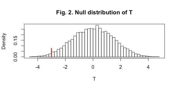
It’s worth noting that the permutation distribution of T in this example looks a lot like a normal distribution, and in fact, as the number of pairs grows large, it will resemble a normal distribution more and more. But had the number of pairs been smaller, or the observed distributions of differences more skewed, the normal approximation would not be as good, but inferences from the simulated permutation distribution would remain just as valid as before.
Bio: Shane Pederson is a Senior Data Scientist at Open Data Group in Chicago, where he consults on a variety of big- and small-data engagements. He has worked as a consulting statistician for over 30 years – in government (Los Alamos National Laboratory), academics (Georgia Institute of Technology) and banking (JPMorgan Chase). He has extensive experience in engineering, litigation and econometrics, and has received several patents relating to the optimization of financial services analytics. He is a native Minnesotan and received his BS and PhD degrees in Statistics from the University of Minnesota.
Related: