Why physical storage of your database tables might matter
Follow this investigation into why physical storage of your database tables might matter, from problem identification to possible issue resolutions.
By Apoorva Aggarwal, Machine Learning and Data Engineer at Grofers

In our quest to simplify and enrich online grocery shopping for our users, we experimented with serving personalized item recommendations to each one of them. For this we operated in batch mode and pre computed relevant top 200 item recommendations for each user and dumped the results in a table of our OLTP PostgreSQL database to enable us to serve these recommendations in real time. Queries on this table were taking too long which resulted in bad user experience.
Narrowing down into problem space
Recommendations were pre computed for all users who have ever transacted on our platform, the size of this table was close to 12 GB. A simple SELECT query was used to retrieve recommendations from this table.
db=> SELECT *
FROM personalized_recommendations
WHERE customer_id = 1;
...
db=> \d personalized_recommendations
           Table "public.personalized_recommendations"
    Column    |       Type       | Collation | Nullable | Default
--------------+------------------+-----------+----------+---------
 customer_id  | integer          |           | not null |
 product_id   | integer          |           | not null |
 score        | double precision |           | not null |
 ...
Indexes:
    "personalized_recommendations_temp_customer_id_idx1" btree (customer_id)
A BTree index on column customer_id was created to enable faster lookups. But even then, sometimes query times were as large as ~1 s.
Looking at the query plan :
EXPLAIN ANALYZE
SELECT *
FROM personalized_recommendations
WHERE customer_id = 25001;

QUERY PLAN
— — — — — — — — — — — — —
Index Scan using personalized_recommendations_temp_customer_id_idx on personalized_recommendations (cost=0.57..863.90 rows=214 width=38) (actual time=10.372..110.246 rows=201 loops=1)
 Index Cond: (customer_id = 25001)
Planning time: 0.066 ms
Execution time: 110.335 ms
Isolating the cause
Even though the query planner was using the created index, query times were still huge.This required us to dig deeper into what does having an “index” really mean? How does having an index help in faster fetching of query results? Lets revisit the basic anatomy of an index.
Default index in postgres is of type BTree which constitutes a BTree or a balanced tree of index entries and index leaf nodes which store physical address of an index entry.
An index lookup requires three steps:
- Tree traversal
- Following the leaf node chain
- Fetching the table data
The above steps are explained in detail here.
Tree traversal is the only step that has an upper bound for the number of accessed blocks — the index depth. The other two steps might need to access many blocks — their upper bound can be as large as the full table scan.¹
An Index Scan performs a B-tree traversal, walks through the leaf nodes to find all matching entries, and fetches the corresponding table data. It is like an INDEX RANGE SCAN followed by a TABLE ACCESS BY INDEX ROWIDoperation.
Following the leaf node chain requires getting ROWID’s that fulfill the customer_id condition: in our case, it has max limit of 200 row ID’s. Since these index leaf nodes are stored in a sorted manner, their access is upper bounded by the length of this chain or total rows in the table.
The next step is the TABLE ACCESS BY INDEX ROWID operation. It uses the ROWID from previous step to fetch the rows — all columns — from the table. Here the db engine must fetch the rows individually hitting each record in page and bringing them in memory for retrieval. It involves random access IO’s apart from read operations.
We decided it might be worthwhile to look at how these query result rows were distributed on physical memory. In postgres, location of a row is given by ctidwhich is a tuple. ctid is of type tid (tuple identifier), called ItemPointer in the C code. Per documentation:
This is the data type of the system column ctid. A tuple ID is a pair (block number, tuple index within block) that identifies the physical location of the row within its table.
The distribution was like this:
customer_id | product_id | ctid
 — — — — — — -+ — — — — — —
 1254 | 284670 | (3789,28)
 1254 | 18934 | (7071,73)
 1254 | 14795 | (8033,19)
 1254 | 10908 | (9591,60)
 1254 | 95032 | (11017,83)
 1254 | 318562 | (11134,65)
 1254 | 18854 | (11275,54)
 1254 | 109943 | (11827,76)
 1254 | 105 | (16309,104)
 1254 | 3896 | (18432,8)
 1254 | 3890 | (20062,90)
 1254 | 318550 | (20488,84)
 1254 | 37261 | (20585,62)
 ...
Clearly, rows for a particular customer id were far from each other on disk. This seemed to explain the high execution times of queries having customer_id in WHERE clause. The db engine was hitting pages on disk for retrieving each row. There was high random access IO. What if we could bring all rows of a particular customer together? If done, the engine might be able to retrieve all rows in result set in one go.
Possible solutions to root cause and exploring feasibility
Postgres provides a CLUSTER command which physically rearranges the rows on disk based on a given column. But given constraints like acquiring a READ WRITE lock on table and requiring 2.5x the table size made it tricky to use. We began to explore if we could write the table in customer id rows sorted manner. The application which was writing these rows was a Spark application using collaborative filtering algorithm to derive recommended products.
An attempt to fix the problem right from the source
Understanding how Spark writes data to table
The problem required us to dig deeper into how Spark writes to Postgres. It writes data partition wise. Now, what is this partition?
Spark being a distributed computing frame work distributes a particular data frame into partitions amongst its workers. It allows you to explicitly partition a dataframe based on a partition key to ensure minimal shuffling (bring partitions from one worker to another for reading/writing operations). Looking at the code we found that we had partitioned on product_id for a particular transformation operation.
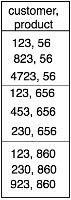
This meant that the data written to our postgres table should be product_idwise, i.e. rows of all customer ID’s whose recommendations were a particular product ID should be clubbed together. We tested our hypothesis by looking at results of :
SELECT *, ctid FROM personalized_recommendations WHERE product_id = 284670
 product_id | customer_id |   ctid
------------+-------------+----------
     284670 |        1133 | (479502,71)
     284670 |        2488 | (479502,72)
     284670 |        3657 | (479502,73)
     284670 |        2923 | (479502,74)
     284670 |        6911 | (479502,75)
     284670 |        9018 | (479502,76)
     284670 |        4263 | (479502,77)
     284670 |        1331 | (479502,78)
     284670 |        3242 | (479502,79)
     284670 |        3661 | (479502,80)
     284670 |        9867 | (479502,81)
     284670 |        7066 | (479502,82)
     284670 |       10267 | (479502,83)
     284670 |        7499 | (479502,84)
     284670 |        8011 | (479502,85)
Yes indeed, all rows of a particular product ID were together on the table. So if we instead partitioned on customer_id, our objective of bringing all result rows of a customer_id would be met. This could be achieved by re partitioning the dataframe. This post here talks about repartition in detail.
Attempting to align the data
We repartitioned the dataframe by :
df.repartition($”customer_id”)
And wrote the final dataframe to postgres. Now we checked for distribution of rows.
db=> SELECT product_id,customer_id,ctid FROM personalized_recommendations WHERE customer_id = 28460
limit 20;
 customer_id | product_id | ctid
 — — — — — — + — — — — — — -+ — — — — —
 28460 | 1133 | (0,24)
 28460 | 2488 | (4,7)
 28460 | 3657 | (9,83)
 28460 | 2923 | (18,54)
 28460 | 6911 | (20,42)
 28460 | 9018 | (31,59)
 28460 | 4263 | (35,79)
 28460 | 1331 | (38,14)
 28460 | 3242 | (40,41)
 28460 | 3661 | (55,105)
 28460 | 9867 | (57,21)
 28460 | 7066 | (61,28)
 28460 | 10267 | (62,63)
 28460 | 7499 | (66,8)
Alas, the table is still not pivoted on customer_id. What did we do wrong?
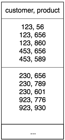
Apparently, the default number of partitions on which data is rearranged is 200. But since the number of distinct customer ID’s were greater than 200 (~10 million), this meant that a single partition will contain recommended products of more that 1 customer as seen in the figure below. In this case, close to (~10 million/200=50,000) customers.
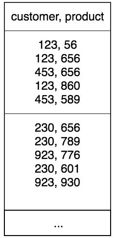
When this particular partition will be written to the db, this will still not ensure that all rows belonging to a customer_id be written together. We then sorted rows within a partition by customer_id:
df.repartition($”customer_id”).sortWithinPartitions($”customer_id”)
It is an expensive operation for spark to perform but nevertheless necessary for us. We did this and wrote again to the database. Next we checked for distribution.
customer_id | product_id | ctid
 — — — — — — -+ — — — — — — + — — — — — -
 1254 | 284670 | (212,95)
 1254 | 18854 | (212,96)
 1254 | 18850 | (212,97)
 1254 | 318560 | (212,98)
 1254 | 318562 | (212,99)
 1254 | 318561 | (212,100)
 1254 | 10732 | (212,101)
 1254 | 108 | (212,102)
 1254 | 11237 | (212,103)
 1254 | 318058 | (212,104)
 1254 | 38282 | (212,105)
 1254 | 3884 | (212,106)
 1254 | 31 | (212,107)
 1254 | 318609 | (215,1)
 1254 | 2 | (215,2)
 1254 | 240846 | (215,3)
 1254 | 197964 | (215,4)
 1254 | 232970 | (215,5)
 1254 | 124472 | (215,6)
 1254 | 19481 | (215,7)
 …
Voila! Its now pivoted on customer_id (tears of joy :,-) ).
Testing the solution
The final test still remains. Will the query execution now be faster. Lets see what the query planner says.
EXPLAIN ANALYZE
SELECT *
FROM personalized_recommendations
WHERE customer_id = 25001;

QUERY PLAN

Bitmap Heap Scan on personalized_recommendations(cost=66.87..13129.94 rows=3394 width=38) (actual time=2.843..3.259 rows=201 loops=1)
 Recheck Cond: (customer_id = 25001)
 Heap Blocks: exact=2
 -> Bitmap Index Scan on personalized_recommendations_temp_customer_id_idx (cost=0.00..66.02 rows=3394 width=0) (actual time=1.995..1.995 rows=201 loops=1)
 Index Cond: (customer_id = 25001)
 Planning time: 0.067 ms
 Execution time: 3.322 ms
Execution time came down from ~100 ms to ~3ms.
This optimization really helped us use personalized recommendations to serve a variety of use cases like generating targeted advertising pushes for a growing consumer base of more than 200 thousand users in bulk etc. When this was first launched, size of the data was ~12 GB. Now in the past 1 year, it has grown to ~22GB but rearranging the records in the table has helped to keep database retrieval latencies to minimal. Although now, the time taken for Spark application to generate these recommendations, arranging the dataframe and writing to database has increased manifold. But since that happens in batch mode, it is still acceptable.
With growing scale of users on the platform, data too is growing daily and so are the challenges to process it and make it useful for data driven decision making. If you like to solve similar problems at scale, we are always looking for new talent. Check for open positions here.
Footnotes:
[1]. https://use-the-index-luke.com/sql/anatomy/slow-indexes
Bio: Apoorva Aggarwal is a Machine Learning and Data Engineer at Grofers.
Originally posted on Grofers Engineering Blog. Reposted with permission.
Related:
- 7 Steps to Mastering SQL for Data Science — 2019 Edition
- Simple Tips for PostgreSQL Query Optimization
- Loading Terabytes of Data from Postgres into BigQuery