 The 10 Statistical Techniques Data Scientists Need to Master
 The 10 Statistical Techniques Data Scientists Need to Master
The author presents 10 statistical techniques which a data scientist needs to master. Build up your toolbox of data science tools by having a look at this great overview post.
Regardless of where you stand on the matter of Data Science sexiness, it’s simply impossible to ignore the continuing importance of data, and our ability to analyze, organize, and contextualize it. Drawing on their vast stores of employment data and employee feedback, Glassdoor ranked Data Scientist #1 in their 25 Best Jobs in America list. So the role is here to stay, but unquestionably, the specifics of what a Data Scientist does will evolve. With technologies like Machine Learning becoming ever-more common place, and emerging fields like Deep Learning gaining significant traction amongst researchers and engineers — and the companies that hire them — Data Scientists continue to ride the crest of an incredible wave of innovation and technological progress.
While having a strong coding ability is important, data science isn’t all about software engineering (in fact, have a good familiarity with Python and you’re good to go). Data scientists live at the intersection of coding, statistics, and critical thinking. As Josh Wills put it, “data scientist is a person who is better at statistics than any programmer and better at programming than any statistician.” I personally know too many software engineers looking to transition into data scientist and blindly utilizing machine learning frameworks such as TensorFlow or Apache Spark to their data without a thorough understanding of statistical theories behind them. So comes the study of statistical learning, a theoretical framework for machine learning drawing from the fields of statistics and functional analysis.
Why study Statistical Learning? It is important to understand the ideas behind the various techniques, in order to know how and when to use them. One has to understand the simpler methods first, in order to grasp the more sophisticated ones. It is important to accurately assess the performance of a method, to know how well or how badly it is working. Additionally, this is an exciting research area, having important applications in science, industry, and finance. Ultimately, statistical learning is a fundamental ingredient in the training of a modern data scientist. Examples of Statistical Learning problems include:
- Identify the risk factors for prostate cancer.
- Classify a recorded phoneme based on a log-periodogram.
- Predict whether someone will have a heart attack on the basis of demographic, diet and clinical measurements.
- Customize an email spam detection system.
- Identify the numbers in a handwritten zip code.
- Classify a tissue sample into one of several cancer classes.
- Establish the relationship between salary and demographic variables in population survey data.
In my last semester in college, I did an Independent Study on Data Mining. The class covers expansive materials coming from 3 books: Intro to Statistical Learning (Hastie, Tibshirani, Witten, James), Doing Bayesian Data Analysis(Kruschke), and Time Series Analysis and Applications (Shumway, Stoffer). We did a lot of exercises on Bayesian Analysis, Markov Chain Monte Carlo, Hierarchical Modeling, Supervised and Unsupervised Learning. This experience deepens my interest in the Data Mining academic field and convinces me to specialize further in it. Recently, I completed the Statistical Learning online course on Stanford Lagunita, which covers all the material in the Intro to Statistical Learning book I read in my Independent Study. Now being exposed to the content twice, I want to share the 10 statistical techniques from the book that I believe any data scientists should learn to be more effective in handling big datasets.
Before moving on with these 10 techniques, I want to differentiate between statistical learning and machine learning. I wrote one of the most popular Medium posts on machine learning before, so I am confident I have the expertise to justify these differences:
- Machine learning arose as a subfield of Artificial Intelligence.
- Statistical learning arose as a subfield of Statistics.
- Machine learning has a greater emphasis on large scale applications and prediction accuracy.
- Statistical learning emphasizes models and their interpretability, and precision and uncertainty.
- But the distinction has become and more blurred, and there is a great deal of “cross-fertilization.”
- Machine learning has the upper hand in Marketing!
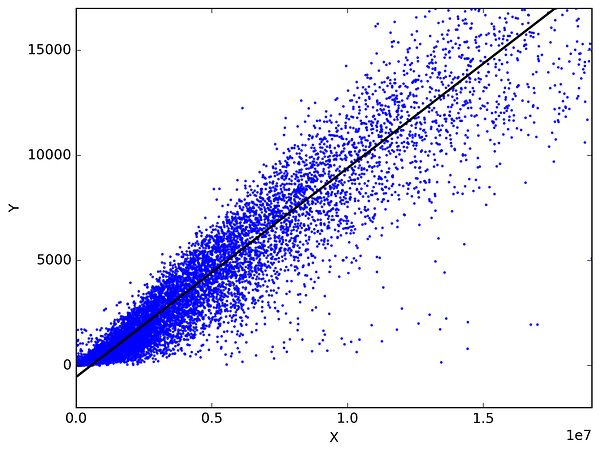
1 — Linear Regression:
In statistics, linear regression is a method to predict a target variable by fitting the best linear relationship between the dependent and independent variable. The best fit is done by making sure that the sum of all the distances between the shape and the actual observations at each point is as small as possible. The fit of the shape is “best” in the sense that no other position would produce less error given the choice of shape. 2 major types of linear regression are Simple Linear Regression and Multiple Linear Regression. Simple Linear Regressionuses a single independent variable to predict a dependent variable by fitting a best linear relationship. Multiple Linear Regression uses more than one independent variable to predict a dependent variable by fitting a best linear relationship.
Pick any 2 things that you use in your daily life and that are related. Like, I have data of my monthly spending, monthly income and the number of trips per month for the last 3 years. Now I need to answer the following questions:
- What will be my monthly spending for next year?
- Which factor (monthly income or number of trips per month) is more important in deciding my monthly spending?
- How monthly income and trips per month are correlated with monthly spending?
2 — Classification:
Classification is a data mining technique that assigns categories to a collection of data in order to aid in more accurate predictions and analysis. Also sometimes called a Decision Tree, classification is one of several methods intended to make the analysis of very large datasets effective. 2 major Classification techniques stand out: Logistic Regression and Discriminant Analysis.
Logistic Regression is the appropriate regression analysis to conduct when the dependent variable is dichotomous (binary). Like all regression analyses, the logistic regression is a predictive analysis. Logistic regression is used to describe data and to explain the relationship between one dependent binary variable and one or more nominal, ordinal, interval or ratio-level independent variables. Types of questions that a logistic regression can examine:
- How does the probability of getting lung cancer (Yes vs No) change for every additional pound of overweight and for every pack of cigarettes smoked per day?
- Do body weight calorie intake, fat intake, and participant age have an influence on heart attacks (Yes vs No)?
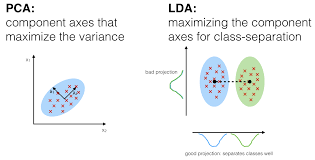
In Discriminant Analysis, 2 or more groups or clusters or populations are known a priori and 1 or more new observations are classified into 1 of the known populations based on the measured characteristics. Discriminant analysis models the distribution of the predictors X separately in each of the response classes, and then uses Bayes’ theorem to flip these around into estimates for the probability of the response category given the value of X. Such models can either be linear or quadratic.
- Linear Discriminant Analysis computes “discriminant scores” for each observation to classify what response variable class it is in. These scores are obtained by finding linear combinations of the independent variables. It assumes that the observations within each class are drawn from a multivariate Gaussian distribution and the covariance of the predictor variables are common across all k levels of the response variable Y.
- Quadratic Discriminant Analysis provides an alternative approach. Like LDA, QDA assumes that the observations from each class of Y are drawn from a Gaussian distribution. However, unlike LDA, QDA assumes that each class has its own covariance matrix. In other words, the predictor variables are not assumed to have common variance across each of the k levels in Y.
3 — Resampling Methods:
Resampling is the method that consists of drawing repeated samples from the original data samples. It is a non-parametric method of statistical inference. In other words, the method of resampling does not involve the utilization of the generic distribution tables in order to compute approximate p probability values.
Resampling generates a unique sampling distribution on the basis of the actual data. It uses experimental methods, rather than analytical methods, to generate the unique sampling distribution. It yields unbiased estimates as it is based on the unbiased samples of all the possible results of the data studied by the researcher. In order to understand the concept of resampling, you should understand the terms Bootstrapping and Cross-Validation:
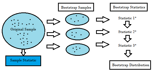
- Bootstrapping is a technique that helps in many situations like validation of a predictive model performance, ensemble methods, estimation of bias and variance of the model. It works by sampling with replacement from the original data, and take the “not chosen” data points as test cases. We can make this several times and calculate the average score as estimation of our model performance.
- On the other hand, cross validation is a technique for validating the model performance, and it’s done by split the training data into k parts. We take the k — 1 parts as our training set and use the “held out” part as our test set. We repeat that k times differently. Finally, we take the average of the k scores as our performance estimation.
Usually for linear models, ordinary least squares is the major criteria to be considered to fit them into the data. The next 3 methods are the alternative approaches that can provide better prediction accuracy and model interpretability for fitting linear models.
4 — Subset Selection:
This approach identifies a subset of the p predictors that we believe to be related to the response. We then fit a model using the least squares of the subset features.
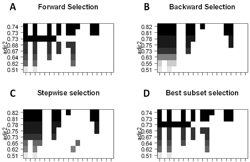
- Best-Subset Selection: Here we fit a separate OLS regression for each possible combination of the p predictors and then look at the resulting model fits. The algorithm is broken up into 2 stages: (1) Fit all models that contain k predictors, where k is the max length of the models, (2) Select a single model using cross-validated prediction error. It is important to use testing or validation error, and not training error to assess model fit because RSS and R² monotonically increase with more variables. The best approach is to cross-validate and choose the model with the highest R² and lowest RSS on testing error estimates.
- Forward Stepwise Selection considers a much smaller subset of ppredictors. It begins with a model containing no predictors, then adds predictors to the model, one at a time until all of the predictors are in the model. The order of the variables being added is the variable, which gives the greatest addition improvement to the fit, until no more variables improve model fit using cross-validated prediction error.
- Backward Stepwise Selection begins will all p predictors in the model, then iteratively removes the least useful predictor one at a time.
- Hybrid Methods follows the forward stepwise approach, however, after adding each new variable, the method may also remove variables that do not contribute to the model fit.
5 — Shrinkage:
This approach fits a model involving all p predictors, however, the estimated coefficients are shrunken towards zero relative to the least squares estimates. This shrinkage, aka regularization has the effect of reducing variance. Depending on what type of shrinkage is performed, some of the coefficients may be estimated to be exactly zero. Thus this method also performs variable selection. The two best-known techniques for shrinking the coefficient estimates towards zero are the ridge regression and the lasso.
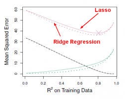
- Ridge regression is similar to least squares except that the coefficients are estimated by minimizing a slightly different quantity. Ridge regression, like OLS, seeks coefficient estimates that reduce RSS, however they also have a shrinkage penalty when the coefficients come closer to zero. This penalty has the effect of shrinking the coefficient estimates towards zero. Without going into the math, it is useful to know that ridge regression shrinks the features with the smallest column space variance. Like in prinicipal component analysis, ridge regression projects the data into ddirectional space and then shrinks the coefficients of the low-variance components more than the high variance components, which are equivalent to the largest and smallest principal components.
- Ridge regression had at least one disadvantage; it includes all p predictors in the final model. The penalty term will set many of them close to zero, but never exactly to zero. This isn’t generally a problem for prediction accuracy, but it can make the model more difficult to interpret the results. Lasso overcomes this disadvantage and is capable of forcing some of the coefficients to zero granted that s is small enough. Since s = 1 results in regular OLS regression, as s approaches 0 the coefficients shrink towards zero. Thus, Lasso regression also performs variable selection.