Choosing the Right Clustering Algorithm for Your Dataset
Applying a clustering algorithm is much easier than selecting the best one. Each type offers pros and cons that must be considered if you’re striving for a tidy cluster structure.
Data clustering is an essential step in the arrangement of a correct and throughout data model. To fulfill an analysis, the volume of information should be sorted out according to the commonalities. The main question is, what commonality parameter provides the best results – and what is implicated under “the best” definition at all.
This article should be useful for the beginning data scientists, or for experts who want to refresh their memories on the topic. It includes the most widespread clustering algorithms, as well as their insightful review. Depending on the particularities of each method, the recommendations considering their application are provided.
Four Basic Algorithms And How To Choose One
Depending on the clusterization models, four common classes of algorithms are differentiated. There are no less than 100 algorithms in general, but their popularity is rather moderate, as well as their field of application.
Connectivity-based Clustering
Clusterization, based on the computation of distances between the objects of the whole dataset, is called connectivity-based, or hierarchical. Depending on the “direction” of the algorithm, it can unite or, inversely, divide the array of information – the names agglomerative and divisive appeared from this exact variation. The most popular and reasonable type is the agglomerative one, where you start by inputting the number of data points, that then are subsequently united into larger and larger clusters, until the limit is reached.
The most prominent example of connectivity-based clusterization is the classification of plants. The “tree” of dataset starts with a particular species and ends with a few kingdoms of plants, each consisting of even smaller clusters (phyla, classes, orders, etc.)
After applying one of the connectivity-based algorithms you receive a dendrogram of data, that presents you the structure of the information rather than its distinct separation on clusters. Such a feature may possess both the benefit or the harm: the complexity of the algorithm may turn out to be excessive or simply inapplicable for datasets with little to no hierarchy. It also shows poor performance: due to the abundance of iterations, complete processing will take an unreasonable amount of time. On top of that, you won’t get a precise structure using the hierarchical algorithm.
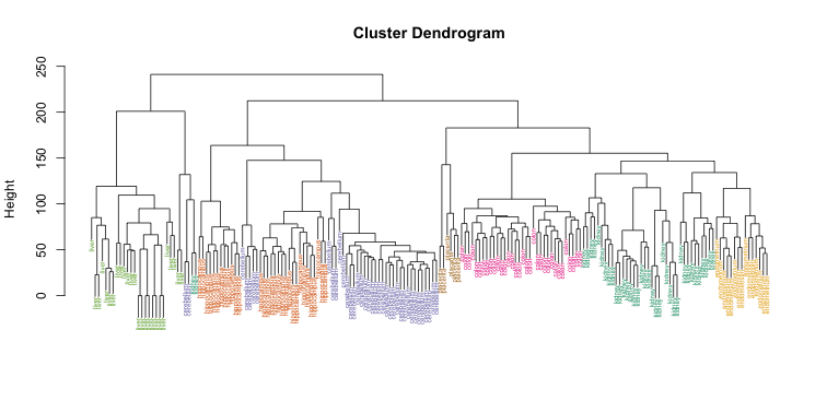
Image source
At the same time, the incoming data required from the counter comes down to the number of data points, that doesn’t influence the final result substantially, or the preset distance metric, that is coarse-measured and approximate as well.
Centroid-based Clustering
Centroid-based clustering, from my experience, is the most frequently occurred model thanks to its comparative simplicity. The model is aimed at classifying each object of the dataset to the particular cluster. The number of clusters (k) is chosen randomly, which is probably the greatest “weakness” of the method. This k-means algorithm is especially popular in machine learning thanks to the alikeness with k-nearest neighbors (kNN) method.
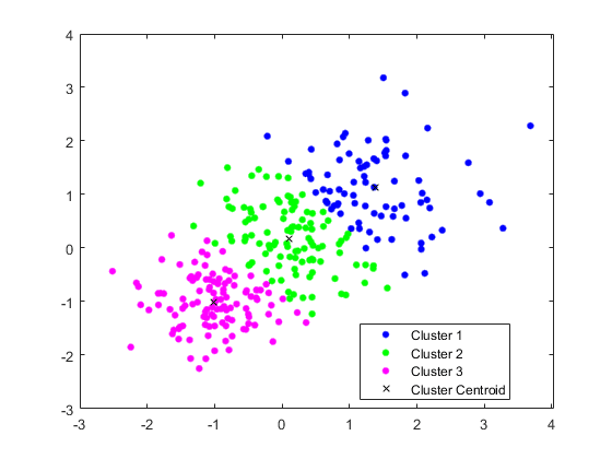
Image source
The process of calculation consists of multiple steps. Firstly, the incoming data is chosen, which is the rough number of the clusters the dataset should be divided into. The centers of clusters should be situated as far as possible from each other – that will increase the accuracy of the result.
Secondly, the algorithm finds distances between each object of the dataset and every cluster. The smallest coordinate (if we’re talking about graphical representation) determines to which cluster the object is moved.
After that, the center of the cluster is recalculated according to the means of all objects’ coordinates. The first step of the algorithm repeats, but with a new center of the cluster that was recomputed. Such iterations continue unless certain conditions are reached. For example, the algorithm may end when the center of the cluster hasn’t moved or moved insignificantly from the previous iteration.
Despite the simplicity – both mathematical and coding – k-means has some drawbacks that don’t allow me to use it everywhere possible. That includes:
- a negligent edge of each cluster, because the priorities are set on the center of the cluster, not on its borders;
- an inability to create a structure of a dataset with objects that can be classified to multiple clusters in equal measure;
- a need to guess the optimal k number, or a need to make preliminary calculations to specify this gauge.
Expectation-maximization Clustering
Expectation-maximization algorithm, at the same time, allows avoiding those complications while providing an even higher level of accuracy. Simply put, it calculates the relation probability of each dataset point to all the clusters we’ve specified. The main “tool” that is used for this clusterization model is Gaussian Mixture Models (GMM) – the assumption that the points of the dataset generally follow the Gaussian distribution.
The k-means algorithm is, basically, a simplified version of the EM principle. They both require manual input of clusters number, and that’s the main intricacy the methods bear. Apart from that, the principles of computing (either for GMM or k-means) are simple: the approximate range of cluster is specified gradually with each new iteration.
Unlike the centroid-based models, the EM algorithm allows the points to classify for two or more clusters – it simply presents you the possibility of each event, using which you’re able to conduct further analysis. More to that, the borders of each cluster compose ellipsoids of different measures unlike k-means, where the cluster is visually represented as a circle. However, the algorithm simply would not work for datasets where objects do not follow the Gaussian distribution. That is the main disadvantage of the method: it is more applicable to theoretical problems rather than the actual measurements or observations.
Density-based Clustering
Finally, the unofficial favorite of data scientists’ hearts, density-based clustering comes. The name comprises the main point of the model – to divide the dataset into clusters the counter inputs the ε parameter, the “neighborhood” distance. If the object is located within the circle (sphere) of the ε radius, it, therefore, relates to the cluster.
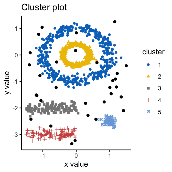
Image source
Step by step, DBSCAN (Density-Based Spatial Clustering of Applications with Noise) algorithm checks every object, changes its status to “viewed,” classifies it to the cluster OR noise, until finally the whole dataset is processed. The clusters determined with DBSCAN can have arbitrary shapes, thereby are extremely accurate. Besides, the algorithm doesn’t make you calculate the number of clusters – it is determined automatically.
Still, even such a masterpiece as DBSCAN has a drawback. If the dataset consists of variable density clusters, the method shows poor results. It also might not be your choice if the placement of objects is too close, and the ε parameter can’t be estimated easily.
Summary
Summing up, there is no such thing as a wrong-chosen algorithm – some of them are just more suitable for the particular dataset structures. In order to always pick up the best (read – more suitable) algorithm, you need to have a throughout understanding of their advantages, disadvantages, and peculiarities.
Some algorithms could be excluded from the very beginning if they, for example, do not correspond with the dataset specifications. To avoid odd work, you can spend a little time memorizing the information instead of choosing the path of trial and error and learning from your own mistakes.
We wish you to always pick the best algorithm at first. Keep up the great job!
Josh Thompson is a Lead Editor at Masters in Data Science. He is in charge of writing case studies, how-tos, and blog posts on AI, ML, Big Data, and hard work of data specialists. In his leisure time, he adores swimming and motorcycling.