Introduction to Geographical Time Series Prediction with Crime Data in R, SQL, and Tableau
When reviewing geographical data, it can be difficult to prepare the data for an analysis. This article helps by covering importing data into a SQL Server database; cleansing and grouping data into a map grid; adding time data points to the set of grid data and filling in the gaps where no crimes occurred; importing the data into R; running XGBoost model to determine where crimes will occur on a specific day
By Jason Wittenauer, Lead Data Scientist at Huron Consulting Group

In this tutorial you will learn how to prepare geographical data for time series predictions.
When reviewing geographical data, it can be difficult to prepare the data for an analysis. There are specific algorithms that can be used, but they can be limited in what they do. If we spend some time splitting up the data into grids and then adding a time point for each grid point, it opens up more possibilities for modeling algorithms and other features that can be added. However, it does create an issue with the size of the data set.
A five year crime data set can easily consist of 250,000 records. Once that is extrapolated into a time series grid of an entire city, it can easily hit 75 million data points. When dealing with data of this size, it is helpful to use a database to cleanse the data before sending it to a modeling script. The steps we will follow are listed below:
- Importing data into a SQL Server database.
- Cleansing and grouping data into a map grid.
- Adding time data points to the set of grid data and filling in the gaps where no crimes occurred.
- Importing the data into R
- Running an XGBoost model to determine where crimes will occur on a specific day
At the end, we will discuss the next steps for making the predictions more usable to end users in BI tools like Tableau.
Prerequisites
Before beginning this tutorial, you will need:
- SQL Server Express installed
- SQL Management Studio or similar IDE to interface with SQL Server
- R installed
- R Studio, Jupyter notebook, or other IDE to interface with R
- A general working knowledge of SQL and R
Data Flow Overview
We will be keeping the database and data flow in a simple structure for now. The database itself will be very flat and the final data handoff into the Tableau dashboard will be executed via a text file. In a more production ready version, we would be saving the predictions back into the database and pulling from that database into the reporting dashboard. For this example, we are not triyng to architect everything perfectly, but just understand the basics of doing geographical time series predictions.
Our data flow is below:

Setup the Database
Our prediction model will be using crime data for the Baltimore area from 2012 to 2017. This is located in the "Data" folder within this repo and the filename is "Baltimore Incident Data.zip". Before importing this data you will need to follow one of the options below to setup the database:
Option 1
- Restore a SQL database using the backup file located in the "Database Objects\Clean Backup\" folder.
Option 2
- Use the scripts located in the "Database Objects" folder under "Tables" and "Procedures" to manually create all of the objects.
Import the Data
Once the database has been successfully created, you can now import the data. This will require you to do the following:
- Unzip the "Baltimore Incident Data.zip" file found in the "Data" folder.
- Run the "Insert_StagingCrime" procedure and make sure it is pointed to the correct import file and to the correct format file (found in the "Data" folder named "FormatFile.fmt").
EXEC Insert_StagingCrime
This procedure will be truncating the Staging_Crime and inserting data from the file directly into it using a BULK INSERT. The staging table itself has all VARCHAR(MAX) data types which we will convert into better data types in the next phase of the import process. A code snippet of the procedure is below.
BULK INSERT Staging_Crime
FROM 'C:\Projects\Crime Prediction\Data\Baltimore Incident Data.csv'
WITH (FIRSTROW = 2, FORMATFILE = 'C:\Projects\Crime Prediction\Data\FormatFile.fmt')
Review the Data.
Now that the data has been imported into the staging table, you can view it by running the below code in SQL Management Studio:
SELECT TOP 10 *
FROM [dbo].[Staging_Crime]
Giving you the following results.
| CrimeDate | CrimeTime | CrimeCode | Address | Description | InsideOutside | Weapon | Post | District | Neighborhood | Location | Premise | TotalIncidents |
|---|---|---|---|---|---|---|---|---|---|---|---|---|
| 02/28/2017 | 23:50:00 | 6D | 2400 KEYWORTH AVE | LARCENY FROM AUTO | O | NULL | 533 | NORTHERN | Greenspring | (39.3348700000, -76.6590200000) | STREET | 1 |
| 02/28/2017 | 23:36:00 | 4D | 200 DIENER PL | AGG. ASSAULT | I | HANDS | 843 | SOUTHWESTERN | Irvington | (39.2830300000, -76.6878200000) | APT/CONDO | 1 |
| 02/28/2017 | 23:02:00 | 4E | 1800 N MOUNT ST | COMMON ASSAULT | I | HANDS | 742 | WESTERN | Sandtown-Winchester | (39.3092400000, -76.6449800000) | ROW/TOWNHO | 1 |
| 02/28/2017 | 23:00:00 | 6D | 200 S CLINTON ST | LARCENY FROM AUTO | O | NULL | 231 | SOUTHEASTERN | Highlandtown | (39.2894600000, -76.5701900000) | STREET | 1 |
| 02/28/2017 | 22:00:00 | 6E | 1300 TOWSON ST | LARCENY | O | NULL | 943 | SOUTHERN | Locust Point | (39.2707100000, -76.5911800000) | STREET | 1 |
| 02/28/2017 | 21:40:00 | 6J | 1000 WILMOT CT | LARCENY | O | NULL | 312 | EASTERN | Oldtown | (39.2993600000, -76.6034100000) | STREET | 1 |
| 02/28/2017 | 21:40:00 | 6J | 2400 PENNSYLVANIA AVE | LARCENY | O | NULL | 733 | WESTERN | Penn North | (39.3094200000, -76.6417700000) | STREET | 1 |
| 02/28/2017 | 21:30:00 | 5D | 1500 STACK ST | BURGLARY | I | NULL | 943 | SOUTHERN | Riverside | (39.2721500000, -76.6033600000) | OTHER/RESI | 1 |
| 02/28/2017 | 21:30:00 | 6D | 2100 KOKO LN | LARCENY FROM AUTO | O | NULL | 731 | WESTERN | Panway/Braddish Avenue | (39.3117800000, -76.6633200000) | STREET | 1 |
| 02/28/2017 | 21:10:00 | 3CF | 800 W LEXINGTON ST | ROBBERY - COMMERCIAL | O | FIREARM | 712 | WESTERN | Poppleton | (39.2910500000, -76.6310600000) | STREET | 1 |
Notice how this data has the point in time the crime occurred, the latitude/longitude, and even crime categories. Those categories can be very useful for more advanced modeling techniques and analytics.
Cleanse the Data and Create Grids of the Map
Next we can move our data into a "Crime" table that has the correct data types associated with it. During this step we will also split out the location field into longitude and latitude fields. All of the logic to complete these steps can be done by running the below execution statement:
EXEC Insert_Crime
And now we will have data populating the "Crime" table. This will allow us to complete the next step to create a grid on the city and assign each crime to one of the grid squares. You will notice that we create two grids (small and large). This allows us to create features that are at the crime location and a little bit further away from the crime location. Essentially giving us hotspots of crime throughout the city.

Run the below code to create the grids and assign a SmallGridID and LargeGridID to the "Crimes" table:
EXEC Update_CrimeCoordinates
This procedure is doing three separate tasks:
- Creating a small grid of squares on the map within the GridSmall table (Procedure: Insert_GridSmall).
- Creating a large grid of squares on the map within the GridLarge table (Procedure: Insert_GridLarge).
- Assigning all the crime records to a small and large square on the map.
The two procedures that create the grid squares are taking in variables to determine the corners of the map and how many squares we want to have on our map. This is defaulting to a small grid that is 200 by 200 and a large grid that has squares twice as big at 100 by 100.
You can view some of the grid data by running the following:
SELECT TOP 10 c.CrimeId, gs.*
FROM [dbo].[Crime] c
JOIN GridSmall gs
    ON gs.GridSmallId = c.GridSmallId
| CrimeId | GridSmallId | BotLeftLatitude | TopRightLatitude | BotLeftLongitude | TopRightLongitude |
|---|---|---|---|---|---|
| 1 | 31012 | 39.3341282000001 | 39.3349965000001 | -76.6594308000001 | -76.6585152000001 |
| 2 | 19121 | 39.2828985 | 39.2837668 | -76.68873 | -76.6878144 |
| 3 | 25198 | 39.3089475000001 | 39.3098158000001 | -76.6456968000001 | -76.6447812000001 |
| 4 | 20657 | 39.2889766 | 39.2898449 | -76.5706176000001 | -76.5697020000001 |
| 5 | 16212 | 39.269874 | 39.2707423 | -76.5916764000001 | -76.5907608000001 |
| 6 | 22832 | 39.2985279000001 | 39.2993962000001 | -76.6035792000001 | -76.6026636000001 |
| 7 | 25202 | 39.3089475000001 | 39.3098158000001 | -76.6420344000001 | -76.6411188000001 |
| 8 | 16601 | 39.2716106 | 39.2724789 | -76.6035792000001 | -76.6026636000001 |
| 9 | 25781 | 39.3115524000001 | 39.3124207000001 | -76.6640088 | -76.6630932 |
| 10 | 20992 | 39.2907132 | 39.2915815 | -76.6319628000001 | -76.6310472000001 |
Notice how there are two points being calculated for a square, the top right and bottom left points. We don't have to calculate all four points on the square even though there is technically some curve to a real map when draw longitude and latitude lines. When the scale gets small enough, we can just assume that the squares are mostly straight lines
Create Crime Grid and Lag Features
The last step we need to complete is creating the entire grid of the map for all time periods we want to evaulate. In our case, that is one grid point per day to determine if a crime is going to occur. To complete this step, the below procedure needs to be executed:
EXEC Insert_CrimeGrid
During this step each crime will be grouped together on the map squares so we can determine when and how many crimes occurred on each date in our data set. We will also need to calculate all the filler dates for each square when no crime occurred to make a complete data set.
The procedure take quite awhile to run. On my laptop, it ran for about 1 hour and the subsequent table ("CrimeGrid") contains about 75 million records. The nice part is that the output is now saved into a table, so we will not have to run it in our R script where large data operations might not run as efficiently as inside a database.
Also during this step we will be creating "lag features". These will be columns that tell us how many times within the last day, two days, week, month, etc. that a crime occured on the grid square. This is essentially helping us do a "hotspot" analysis of the data, which can be used to look at other grid squares nearby to see if the crime is localized to our single square or if it is clustered to all nearby squares, similar to aftershocks in an earthquake. These features may or may not be necessary depending on the type of modeling you do.

Prediction Setup
With all of the data cleansing and feature engineering being done on the database side, the code for doing predictions is quite simple. In our example we will be using XGBoost in R to analyze five years of training data to predict future crimes.
To start, we load our libraries.
# Load required libraries
library(RODBC)
library(xgboost)
library(ROCR)
library(caret)
Loading required package: gplots

Attaching package: 'gplots'

The following object is masked from 'package:stats':

    lowess

Loading required package: lattice
Loading required package: ggplot2
Registered S3 methods overwritten by 'ggplot2':
  method         from
  [.quosures     rlang
  c.quosures     rlang
  print.quosures rlang
Then import the data into R directly from the database. You could also export the data to text files and read in CSV data if that is your preferred method. The queries to pull the data are just written as SQL statements with some date limiters. These could be re-written to pull directly from reporting stored procedures with date parameters for a more productionized version of the code.
# Set seed
set.seed(1001)

# Read in data
dbhandle <- odbcDriverConnect('driver={SQL Server};server=DESKTOP-VLN71V7\\SQLEXPRESS;database=crime;trusted_connection=true')

train <- sqlQuery(dbhandle, 'select IncidentOccurred as target, GridSmallId, GridLargeId, DayOfWeek, MonthOfYear, DayOfYear, Year, PriorIncident1Day, PriorIncident2Days, PriorIncident3Days, PriorIncident7Days, PriorIncident14Days, PriorIncident30Days, PriorIncident1Day_Large, PriorIncident2Days_Large, PriorIncident3Days_Large, PriorIncident7Days_Large, PriorIncident14Days_Large, PriorIncident30Days_Large from crimegrid where crimedate <= \'2/20/2017\' and crimedate >= \'6/1/2012\'')
test <- sqlQuery(dbhandle, 'select IncidentOccurred as target, GridSmallId, GridLargeId, DayOfWeek, MonthOfYear, DayOfYear, Year, PriorIncident1Day, PriorIncident2Days, PriorIncident3Days, PriorIncident7Days, PriorIncident14Days, PriorIncident30Days, PriorIncident1Day_Large, PriorIncident2Days_Large, PriorIncident3Days_Large, PriorIncident7Days_Large, PriorIncident14Days_Large, PriorIncident30Days_Large from crimegrid where crimedate >= \'2/21/2017\' and crimedate <= \'2/27/2017\'')

# Convert integers to numeric for DMatrix
train[] <- lapply(train, as.numeric)
test[] <- lapply(test, as.numeric)

head(train)
| target | GridSmallId | GridLargeId | DayOfWeek | MonthOfYear | DayOfYear | Year | PriorIncident1Day | PriorIncident2Days | PriorIncident3Days | PriorIncident7Days | PriorIncident14Days | PriorIncident30Days | PriorIncident1Day_Large | PriorIncident2Days_Large | PriorIncident3Days_Large | PriorIncident7Days_Large | PriorIncident14Days_Large | PriorIncident30Days_Large |
|---|---|---|---|---|---|---|---|---|---|---|---|---|---|---|---|---|---|---|
| 0 | 3780 | 990 | 5 | 9 | 262 | 2013 | 0 | 0 | 0 | 0 | 0 | 0 | 0 | 0 | 0 | 0 | 0 | 0 |
| 0 | 3781 | 991 | 5 | 9 | 262 | 2013 | 0 | 0 | 0 | 0 | 0 | 0 | 0 | 0 | 0 | 0 | 0 | 0 |
| 0 | 3782 | 991 | 5 | 9 | 262 | 2013 | 0 | 0 | 0 | 0 | 0 | 0 | 0 | 0 | 0 | 0 | 0 | 0 |
| 0 | 3783 | 992 | 5 | 9 | 262 | 2013 | 0 | 0 | 0 | 0 | 0 | 0 | 0 | 0 | 0 | 0 | 0 | 0 |
| 0 | 3784 | 992 | 5 | 9 | 262 | 2013 | 0 | 0 | 0 | 0 | 0 | 0 | 0 | 0 | 0 | 0 | 0 | 0 |
| 0 | 3785 | 993 | 5 | 9 | 262 | 2013 | 0 | 0 | 0 | 0 | 0 | 0 | 0 | 0 | 0 | 0 | 0 | 0 |
Notice in the test data set we are pull 7 days worth of data to test at once, but still keeping the features coming in as if we knew what happened the prior day. This is just so we can test 7 days at once and see how multiple days worth of predictions look in our reporting at the very end.
Another item to note is that the features labeled "_Large" are for the larger grid vs. the smaller grid.
Create Feature Set and Model Parameters
We are defining the features as all of the columns that come after the first "target" column in the SQL query. These are passed in as part of the labeling on the train and test data sets.
# Get feature names (all but first column which is the target)
feature.names <- names(train)[2:ncol(train)]

print(feature.names)

# Make train and test matrices
dtrain <- xgb.DMatrix(data.matrix(train[,feature.names]), label=train$target)
dtest <- xgb.DMatrix(data.matrix(test[,feature.names]), label=test$target)
 [1] "GridSmallId"               "GridLargeId"
 [3] "DayOfWeek"                 "MonthOfYear"
 [5] "DayOfYear"                 "Year"
 [7] "PriorIncident1Day"         "PriorIncident2Days"
 [9] "PriorIncident3Days"        "PriorIncident7Days"
[11] "PriorIncident14Days"       "PriorIncident30Days"
[13] "PriorIncident1Day_Large"   "PriorIncident2Days_Large"
[15] "PriorIncident3Days_Large"  "PriorIncident7Days_Large"
[17] "PriorIncident14Days_Large" "PriorIncident30Days_Large"
Next, setup the parameters for model training. We are keeping them pretty basic for now. Make sure that the evaluation metric is AUC so we can try to maximize our True Positive Rate. This will prevent police officers from patrolling areas unnecessarily. There could be additional work to cover all predicted areas with clever patrolling, but we are not going to get into it during this tutorial.
# Training parameters
watchlist <- list(eval = dtest, train = dtrain)

param <- list(  objective           = "binary:logistic",
                booster             = "gbtree",
                eta                 = 0.01,
                max_depth           = 10,
                eval_metric         = "auc"
)
Run the Model
Now that everything is setup, we can run the model and see how well it is predicting. Keep in mind that this is using a pretty basic set of features just to demonstrate one way to deal with geographic time series data. While the data sets can get quite large, they are easy to understand and can run fairly quickly when using cloud based services like AWS.
This particular training data set had 70 million rows and took about 30 minutes to complete 67 rounds of evaluation on my laptop.
# Run model
clf <- xgb.train(   params                  = param,
                    data                    = dtrain,
                    nrounds                 = 100,
                    verbose                 = 2,
                    early_stopping_rounds   = 10,
                    watchlist               = watchlist,
                    maximize               = TRUE)
[14:30:32] WARNING: amalgamation/../src/learner.cc:686: Tree method is automatically selected to be 'approx' for faster speed. To use old behavior (exact greedy algorithm on single machine), set tree_method to 'exact'.
[1]	eval-auc:0.858208	train-auc:0.858555
Multiple eval metrics are present. Will use train_auc for early stopping.
Will train until train_auc hasn't improved in 10 rounds.

[2]	eval-auc:0.858208	train-auc:0.858555
[3]	eval-auc:0.858208	train-auc:0.858555
[4]	eval-auc:0.858208	train-auc:0.858556
[5]	eval-auc:0.858208	train-auc:0.858556
[6]	eval-auc:0.858208	train-auc:0.858556
[7]	eval-auc:0.858311	train-auc:0.858997
[8]	eval-auc:0.858311	train-auc:0.858997
[9]	eval-auc:0.858311	train-auc:0.858997
[10]	eval-auc:0.858315	train-auc:0.859000
[11]	eval-auc:0.858436	train-auc:0.859110
[12]	eval-auc:0.858436	train-auc:0.859110
[13]	eval-auc:0.858512	train-auc:0.859157
[14]	eval-auc:0.858493	train-auc:0.859157
[15]	eval-auc:0.858496	train-auc:0.859160
[16]	eval-auc:0.858498	train-auc:0.859160
[17]	eval-auc:0.858498	train-auc:0.859160
[18]	eval-auc:0.858342	train-auc:0.859851
[19]	eval-auc:0.858177	train-auc:0.859907
[20]	eval-auc:0.858228	train-auc:0.859971
[21]	eval-auc:0.858231	train-auc:0.859971
[22]	eval-auc:0.858206	train-auc:0.860695
[23]	eval-auc:0.858207	train-auc:0.860695
[24]	eval-auc:0.858731	train-auc:0.860894
[25]	eval-auc:0.858702	train-auc:0.860844
[26]	eval-auc:0.858607	train-auc:0.860844
[27]	eval-auc:0.858574	train-auc:0.860842
[28]	eval-auc:0.858602	train-auc:0.860892
[29]	eval-auc:0.858576	train-auc:0.860843
[30]	eval-auc:0.858574	train-auc:0.860841
[31]	eval-auc:0.858607	train-auc:0.860893
[32]	eval-auc:0.858578	train-auc:0.860843
[33]	eval-auc:0.858611	train-auc:0.860894
[34]	eval-auc:0.858612	train-auc:0.860895
[35]	eval-auc:0.858614	train-auc:0.860898
[36]	eval-auc:0.858615	train-auc:0.860899
[37]	eval-auc:0.858616	train-auc:0.860897
[38]	eval-auc:0.858573	train-auc:0.860870
[39]	eval-auc:0.858546	train-auc:0.860822
[40]	eval-auc:0.858575	train-auc:0.860872
[41]	eval-auc:0.858622	train-auc:0.860898
[42]	eval-auc:0.858578	train-auc:0.860875
[43]	eval-auc:0.858583	train-auc:0.860870
[44]	eval-auc:0.859223	train-auc:0.861768
[45]	eval-auc:0.859220	train-auc:0.861760
[46]	eval-auc:0.859221	train-auc:0.861760
[47]	eval-auc:0.859099	train-auc:0.861719
[48]	eval-auc:0.859112	train-auc:0.861735
[49]	eval-auc:0.859112	train-auc:0.861735
[50]	eval-auc:0.859094	train-auc:0.861734
[51]	eval-auc:0.859125	train-auc:0.861785
[52]	eval-auc:0.859021	train-auc:0.861771
[53]	eval-auc:0.859028	train-auc:0.861784
[54]	eval-auc:0.859029	train-auc:0.861781
[55]	eval-auc:0.859028	train-auc:0.861784
[56]	eval-auc:0.859035	train-auc:0.861788
[57]	eval-auc:0.859037	train-auc:0.861789
[58]	eval-auc:0.859035	train-auc:0.861775
[59]	eval-auc:0.859035	train-auc:0.861774
[60]	eval-auc:0.859010	train-auc:0.861738
[61]	eval-auc:0.859011	train-auc:0.861739
[62]	eval-auc:0.859039	train-auc:0.861778
[63]	eval-auc:0.859016	train-auc:0.861739
[64]	eval-auc:0.859017	train-auc:0.861741
[65]	eval-auc:0.859018	train-auc:0.861746
[66]	eval-auc:0.859019	train-auc:0.861747
[67]	eval-auc:0.859024	train-auc:0.861755
Stopping. Best iteration:
[57]	eval-auc:0.859037	train-auc:0.861789
The model found the patterns quickly and didn't get too much improvement over each round. This could be enhanced with better model parameters and more features.
Review Importance Matrix
Time to analyze our features to see which ones are rating highly in the model by looking at the importance matrix. This can help us determine whether the new features that we add are really worth it on a large data set (larger data set = extra processing time per feature added).
# Compute feature importance matrix
importance_matrix <- xgb.importance(feature.names, model = clf)

# Graph important features
xgb.plot.importance(importance_matrix[1:10,])

It looks like the model it using a combination of small and large grid features to determine if an incident will occur on the current day. It is interesting that the longer term features seem to be more important, indicating a history of criminal activity in the area and/or surrounding areas.
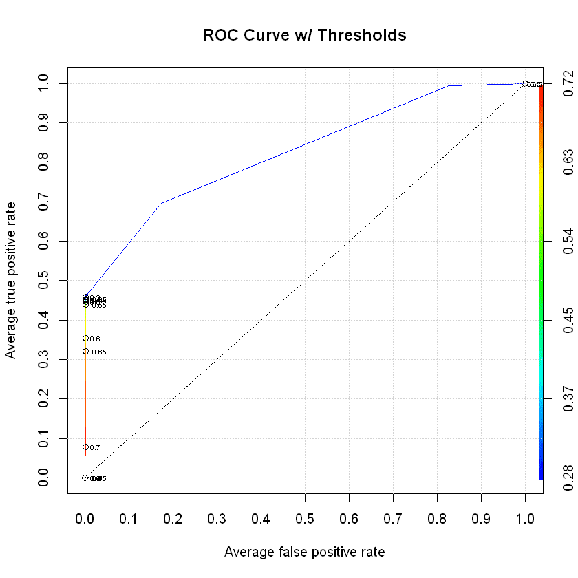
Predict on Test and Check ROC Curve
The last step is to check our predictions against the test data set and see how well they did. We always hope that the ROC curve will spike up really high and really quick, but that is not always the case. In our example, we have a decent score with only basic features included in the model. This definitely shows us that we can do the predictions and more time should be invested to make them better.
# Predict on test data
preds <- predict(clf, dtest)

# Graph AUC curve
xgb.pred <- prediction(preds, test$target)
xgb.perf <- performance(xgb.pred, "tpr", "fpr")

plot(xgb.perf,
     avg="threshold",
     colorize=TRUE,
     lwd=1,
     main="ROC Curve w/ Thresholds",
     print.cutoffs.at=seq(0, 1, by=0.05),
     text.adj=c(-0.5, 0.5),
     text.cex=0.5)
grid(col="lightgray")
axis(1, at=seq(0, 1, by=0.1))
axis(2, at=seq(0, 1, by=0.1))
abline(v=c(0.1, 0.3, 0.5, 0.7, 0.9), col="lightgray", lty="dotted")
abline(h=c(0.1, 0.3, 0.5, 0.7, 0.9), col="lightgray", lty="dotted")
lines(x=c(0, 1), y=c(0, 1), col="black", lty="dotted")
Review the Confusion Matrix
We know there is a decent AUC score but let's look at the actual output of what we predicted vs. what actually happened. The easiest way to do this is to review the confusion matrix. We want the top left and bottom right boxes (good predictions) to be big and the others (bad predictions) to be small.
# Set our cutoff threshold
preds.resp <- ifelse(preds >= 0.5, 1, 0)

# Create the confusion matrix
confusionMatrix(as.factor(preds.resp), as.factor(test$target), positive = "1")
Confusion Matrix and Statistics

          Reference
Prediction      0      1
         0 280581    454
         1     62    367

               Accuracy : 0.9982
                 95% CI : (0.998, 0.9983)
    No Information Rate : 0.9971
    P-Value [Acc > NIR] : < 2.2e-16

                  Kappa : 0.5864

 Mcnemar's Test P-Value : < 2.2e-16

            Sensitivity : 0.447016
            Specificity : 0.999779
         Pos Pred Value : 0.855478
         Neg Pred Value : 0.998385
             Prevalence : 0.002917
         Detection Rate : 0.001304
   Detection Prevalence : 0.001524
      Balanced Accuracy : 0.723397

       'Positive' Class : 1
Over the course of 7 days, it looks like there were 821 incidents and our model correctly predicted 367 of them. The other key point is that we incorrectly predicted 62 incidents, essentially sending police officers to areas where we thought a crime could occur but did not. At face value, this doesn't seem too bad but we would need to see how this affects response times to criminal activity vs. what the current response times are at right now. The idea being that police officers are in areas close enough to a crime that they can either prevent it with their presence or respond to it very quickly to prevent as much harm as possible.
Prepare Data for Reporting
Next we can add in the longitude and latitude coordinates for the test data set and export it to a CSV file. This will allow us to take a look at the actual predictions on a map in a BI tool like Tableau.
# Read in the grid coordinates
gridsmall <- sqlQuery(dbhandle, 'select * from gridsmall')

# Merge the predictions with the test data
results <- cbind(test, preds)

# Merge the grid coordinates with the test data
results <- merge(results, gridsmall, by="GridSmallId")

head(results)

# Save to file
write.csv(results,"Data\\CrimePredictions.csv", row.names = TRUE)
| GridSmallId | target | GridLargeId.x | DayOfWeek | MonthOfYear | DayOfYear | Year | PriorIncident1Day | PriorIncident2Days | PriorIncident3Days | ... | PriorIncident3Days_Large | PriorIncident7Days_Large | PriorIncident14Days_Large | PriorIncident30Days_Large | preds | BotLeftLatitude | TopRightLatitude | BotLeftLongitude | TopRightLongitude | GridLargeId.y |
|---|---|---|---|---|---|---|---|---|---|---|---|---|---|---|---|---|---|---|---|---|
| 1 | 0 | 1 | 3 | 2 | 52 | 2017 | 0 | 0 | 0 | ... | 0 | 0 | 0 | 0 | 0.2822689 | 39.20041 | 39.20128 | -76.71162 | -76.7107 | 1 |
| 1 | 0 | 1 | 5 | 2 | 54 | 2017 | 0 | 0 | 0 | ... | 0 | 0 | 0 | 0 | 0.2822689 | 39.20041 | 39.20128 | -76.71162 | -76.7107 | 1 |
| 1 | 0 | 1 | 7 | 2 | 56 | 2017 | 0 | 0 | 0 | ... | 0 | 0 | 0 | 0 | 0.2822689 | 39.20041 | 39.20128 | -76.71162 | -76.7107 | 1 |
| 1 | 0 | 1 | 4 | 2 | 53 | 2017 | 0 | 0 | 0 | ... | 0 | 0 | 0 | 0 | 0.2822689 | 39.20041 | 39.20128 | -76.71162 | -76.7107 | 1 |
| 1 | 0 | 1 | 2 | 2 | 58 | 2017 | 0 | 0 | 0 | ... | 0 | 0 | 0 | 0 | 0.2822689 | 39.20041 | 39.20128 | -76.71162 | -76.7107 | 1 |
| 1 | 0 | 1 | 1 | 2 | 57 | 2017 | 0 | 0 | 0 | ... | 0 | 0 | 0 | 0 | 0.2822689 | 39.20041 | 39.20128 | -76.71162 | -76.7107 | 1 |
Visualizing the Predictions
It is time to see what these predictions actually look like over the course of 7 days. The Tableau dashboard itself can be found here:
While looking at the predictions that were incorrect (red dots), it looks like they are pretty close to predictions that were correct. This would put police officers in the general vicinity of a crime occurring. So maybe the incorrect predictions are not affecting the overall results very much at all. Example screenshots are shown below with the correct predictions (blue) and incorrect predictions (red).
Incorrect Predictions

Incorrect and Correct Predictions

Overall it does not seem too bad, but we will need more features and/or more data to capture all those missing predictions. Also, there is probably a lot more we can do to focus on specific types of crimes that are occuring and key in on specific prediction modeling to handle each type.
What Next?
This tutorial got us started with doing geographical time series predictions using crime data. We can see that the predictions are definitely working, but there is more work to be done with creating features. We might want to add in some other features that check a larger area for prior crime occurences. Another useful step would be to change our predictions to run hourly and map squad car patrol routes by time of day. Even if the predictions are not perfect, as long as you are putting a police officer in the general vicinity of a crime and it is better than current patrol methodologies, then they can respond much faster or even prevent the crime from occurring in the first place with just their presence.
Other ideas to think about:
- Remove crime data in the vicinity of police stations, fire stations, hospitals, etc. since those could be biased against people submitting reports.
- Add in demographic features related to census information.
- Map crimes to neighborhoods instead of a square grid to predict against.
Hope you enjoyed the tutorial!
Bio: Jason Wittenauer is a data scientist focused on improving hospital earnings with a background in R, Python, Microsoft SQL Server, Tableau, TIBCO Spotfire, and .NET web programming. His areas of focus in healthcare are business operations, revenue improvement, and expense reduction.
Original. Reposted with permission.
Related:
- Stock Market Forecasting Using Time Series Analysis
- What you need to know: The Modern Open-Source Data Science/Machine Learning Ecosystem
- Justice Can’t Be Colorblind: How to Fight Bias with Predictive Policing