Introduction to Statistics for Data Science
Statistics is foundational for Data Science and a crucial skill to master for any practitioner. This advanced introduction reviews with examples the fundamental concepts of inferential statistics by illustrating the differences between Point Estimators and Confidence Intervals Estimates.
By Diogo Menezes Borges, Data Engineer.
In Statistics, to infer the value of an unknown parameter, we use estimators. Estimation is the process used to make inferences, from a sample, about an unknown population parameter.
Based on a random sample of a population, a point estimate is the best estimate, although it is not absolutely accurate. Furthermore, if you continuously retrieve random samples from the same population, it is expected that the point estimate would vary from sample to sample.
On the other hand, a confidence interval is an estimate constructed on the assumption that the true parameter will fall within a specified proportion regardless of the number of samples analysed.
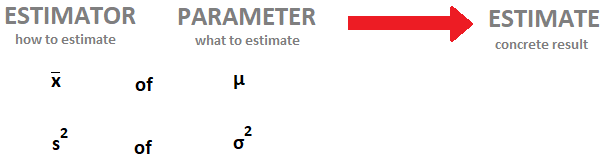
A population estimator is an approximation depending solely on sample information, while on the other hand, a specific value is called an estimate.
As we’ve referred, there are two types of estimates:
- Point Estimates— single number.
- Confidence Interval Estimates — provide much more information, and are preferred when making inferences.
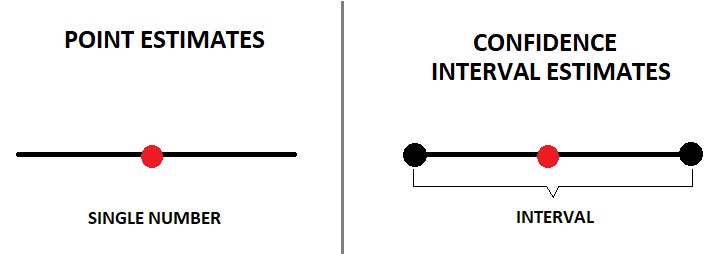
The two are related since the point estimate is in the middle of the confidence interval estimate. However, confidence intervals provide much more information and are preferred when making inferences.
Point Estimates
We’ve seen so far point estimators in earlier posts. For example, the sample mean (x̅) is a point estimation of the population’s mean (μ). The same goes for the sample variance, which is an estimate of the population’s variance.
All estimators have two properties, efficiency and bias:
- Bias— an unbiased estimator has an expected value equal to the population parameter.
- Efficiency — the most efficient estimators are the ones with the least variability of outcomes. The most efficient estimator is the unbiased estimator with the smallest variance.
We’re always looking for the most efficient and unbiased estimators.
Confidence Interval Estimates
Point estimators are not very reliable! A confidence interval is a much more accurate representation of reality. However, there are still some uncertainties left. We can never be 100% confident unless we go through the whole population.
- Example
Imagine you decide to randomly measure 40 men in your city, and you get a sample average height of x̅ =175 cm. You might get close to the population’s real height (μ), but the chances are that the true value is somewhere between 170 cm and 180 cm. It is most accurate to say that the average height for men in your city is somewhere between a specific interval [170 cm, 180 cm].
Nevertheless, there is still some uncertainty left, which we measure in levels of confidence.
For example, we can say that we’re 95% positive that the average men height in our city falls somewhere between 175 cm and 180 cm. Keep in mind that you can never say you are 100% confident since for that you would have to go through the entire population (i.e., all men in the city). Therefore, there is still a 5% chance that the population parameter is outside the expected range.
A confidence interval is a range within which you expect the population parameter to be.
- Confidence Level
It is denoted by 1-α and is called the confidence level of the interval.
α is a value between 0 and 1. Let’s go back to the previous example. If you wish to be 95% confident that our population parameter is inside that interval, α must be 5%. Hence, if we wish a higher level of confidence, for example, 99% then α will be 1%.
- How to calculate the Confidence Interval?
There are two situations when it is possible to calculate the Confidence Interval Estimates:
a) When the population variance is known.
b) When the population variance is unknown.
a) Known Population Variance
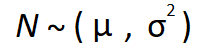
An important factor for this calculation is the assumption that we’re dealing with a population that is Normally Distributed. Even if we’re not dealing with a normal distribution, but we’re working a sample which is large enough, we should take advantage of the Central Limit Theorem to help us out.
It is always simpler to understand these concepts with real-life examples.
- Example
Imagine you wish to become a Data Scientist, and you want to learn how much on average a Data Scientist earns. You got to Glassdoor and start to retrieve salary information from several testimonies. You become aware that the standard deviation (σ) for a Data Scientist salary is around $15,000. Furthermore, make use of the CLT you can assume your sample of 30 salaries (n = 30) are normally distributed.
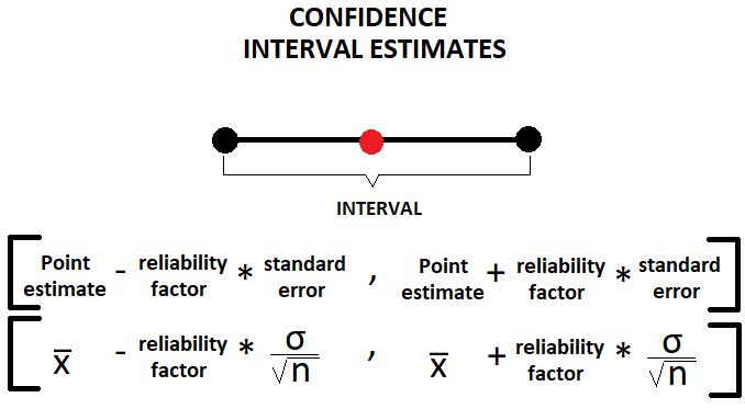
Therefore, assuming a normal distribution, we are able to calculate the confidence interval with a known variance using the following formula:
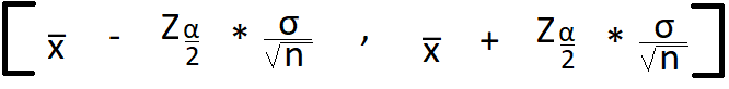
x̅— Sample mean is our point estimator, of $100,200
Z α/2 — Reliability factor, if we assume a confidence level of 95% thus α=5%
σ/sqrt(n) — Standard Error, 15,000/sqrt(30) = $2,739
To get our reliability factor (Z α/2), we have to make use of the z-table for the standard Normal Distribution.
We’ve stated that we’re confident that in 95% of the cases the true population parameter would fall into the specified interval. Hence we must retrieve the reliability factor value of Z 0.05/2 => Z 0.025.
In the table, the value will match the value of 1–0.025=0.975. The corresponding Z comes with the sum of the table row and column associated with that cell.
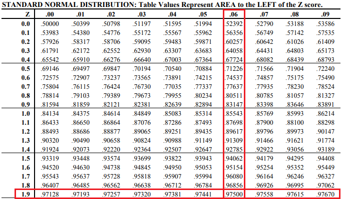
Therefore, for our pratical case, the critical value (commonly used term for Z) for this confidence interval is Z 0.025 = 1.9+0.06 = 1.96.
Therefore, by replacing, each component in the formula we get the following confidence interval.
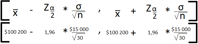
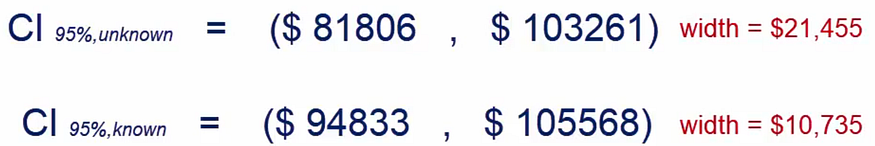
Hence, we’re able to state that we’re 95% sure that the average Data Scientist salary will fall into the specified interval of [$94 883, $105 568]
Now, try it out for a confident interval of 99%. The final result is [$93 135, $107 206].
b) Unknown Population Variance
Until now, we’ve seen how to calculate the confidence interval if the population variance is known. What if it’s not? How should we proceed then? The Student’s Distribution is the answer!
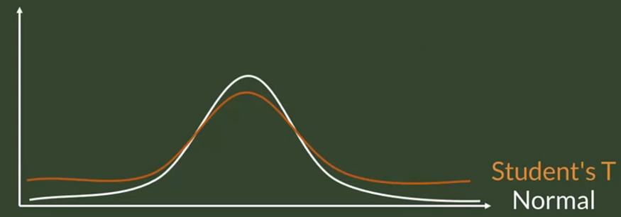
- Student’s T Distribution
The Student’s T Distribution allows inference through small samples for unknown population’s variance. It has a similar shape as the normal distribution but fatter tails which allow for higher dispersion of variables as there is more uncertainty.
Confidence intervals based on small samples, from normally distributed populations, are calculated with the T statistics.
Let’s revisit the example we saw before.
- Example
Again, we look it up in Glassdoor, but this time we only find 9 compensations. We know the sample standard deviation is of $13 932, the sample mean of $92 533 and therefore we can calculate a standard error of $4 644. Nevertheless, we are unaware of the population’s variance. Therefore, we’ll use the Student’s T Distribution!
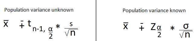
Instead of z statistics, we have t statistics. Moreover, instead of the population standard deviation, we have sample standard deviation (s).
For the Student’s T Distribution, there are n-1 degrees of freedom. Since our sample has n=9 observations, we have 8 degrees of freedom. For this example, we’ll maintain our desirable confidence level of 95% and therefore α = 5%.
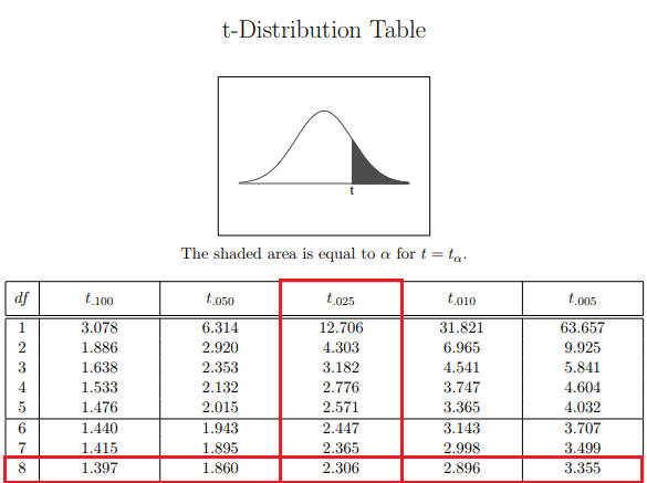
We can conclude that our associated t-statistic is 2,31. Finally, we have all the information needed, so we just need to insert it to the corresponding equation and calculate our confidence interval.
![]()
Therefore, our confidence interval will be of [$81 806, $103 261]. Notice that when comparing our two results, we observe that when we know the population variance, we get a narrower confidence interval. In contrast, when we don’t know the population’s variance, there is a higher uncertainty reflected by wider boundaries for our interval.
In conclusion, what we’ve learned is that when we do not know the population’s variance, we can still make predictions, but they will be less accurate.
Original. Reposted with permission.
Related: