Data Observability, Part II: How to Build Your Own Data Quality Monitors Using SQL
Using schema and lineage to understand the root cause of your data anomalies.
By Barr Moses, CEO and Co-founder of Monte Carlo & Ryan Kearns, Machine Learning Engineer at Monte Carlo
In this article series, we walk through how you can create your own data observability monitors from scratch, mapping to five key pillars of data health. Part I can be found here.
Part II of this series was adapted from Barr Moses and Ryan Kearns’ O’Reilly training, Managing Data Downtime: Applying Observability to Your Data Pipelines, the industry’s first-ever course on data observability. The associated exercises are available here, and the adapted code shown in this article is available here.
As the world’s appetite for data increases, robust data pipelines are all the more imperative. When data breaks — whether from schema changes, null values, duplication, or otherwise — data engineers need to know.
Most importantly, we need to assess the root cause of the breakage — and fast — before it affects downstream systems and consumers. We use “data downtime” to refer to periods of time when data is missing, erroneous, or otherwise inaccurate. If you’re a data professional, you may be familiar with asking the following questions:
- Is the data up to date?
- Is the data complete?
- Are fields within expected ranges?
- Is the null rate higher or lower than it should be?
- Has the schema changed?
To answer these questions in an effective way, we can take a page from the software engineer’s playbook: monitoring and observability.
To refresh your memory since Part I, we define data observability as an organization’s ability to answer these questions and assess the health of their data ecosystem. Reflecting key variables of data health, the five pillars of data observability are:
- Freshness: is my data up to date? Are there gaps in time where my data has not been updated?
- Distribution: how healthy is my data at the field-level? Is my data within expected ranges?
- Volume: is my data intake meeting expected thresholds?
- Schema: has the formal structure of my data management system changed?
- Lineage: if some of my data is down, what is affected upstream and downstream? How do my data sources depend on one another?
In this article series, we’re interested in pulling back the curtain, and investigating what data observability looks like — in the code.
In Part I, we looked at the first two pillars, freshness and distribution, and showed how a little SQL code can operationalize these concepts. These are what we would call more “classic” anomaly detection problems — given a steady stream of data, does anything look out of whack? Good anomaly detection is certainly part of the data observability puzzle, but it’s not everything.
Equally important is context. If an anomaly occurred, great. But where? What upstream pipelines may be the cause? What downstream dashboards will be affected? And has the formal structure of my data changed? Good data observability hinges on our ability to properly leverage metadata to answer these questions — and many others — so we can identify the root cause and fix the issue before it becomes a bigger problem.
In this article, we’ll look at the two data observability pillars designed to give us this critical context — schema and lineage. Once again, we’ll use lightweight tools like Jupyter and SQLite, so you can easily spin up our environment and try these exercises out yourself. Let’s get started.
Our Data Environment
This tutorial is based on Exercises 2 and 3 of our O’Reilly course, Managing Data Downtime. You’re welcome to try out these exercises on your own using a Jupyter Notebook and SQL. We’ll be going into more detail, including exercise 4, in future articles.
If you read Part I of this series, you should be familiar with our data. As before, we’ll work with mock astronomical data about habitable exoplanets. We generated the dataset with Python, modeling data and anomalies off of real incidents I’ve come across in production environments. This dataset is entirely free to use, and the utils folder in the repository contains the code that generated the data, if you’re interested.
I’m using SQLite 3.32.3, which should make the database accessible from either the command prompt or SQL files with minimal setup. The concepts extend to really any query language, and these implementations can be extended to MySQL, Snowflake, and other database environments with minimal changes.
Once again, we have our EXOPLANETS table:
$ sqlite3 EXOPLANETS.db
sqlite> PRAGMA TABLE_INFO(EXOPLANETS);
0 | _id            | TEXT | 0 | | 0
1 | distance       | REAL | 0 | | 0
2 | g              | REAL | 0 | | 0
3 | orbital_period | REAL | 0 | | 0
4 | avg_temp       | REAL | 0 | | 0
5 | date_added     | TEXT | 0 | | 0
A database entry in EXOPLANETS contains the following information:
0. _id: A UUID corresponding to the planet.
1. distance: Distance from Earth, in lightyears.
2. g: Surface gravity as a multiple of g, the gravitational force constant.
3. orbital_period: Length of a single orbital cycle in days.
4. avg_temp: Average surface temperature in degrees Kelvin.
5. date_added: The date our system discovered the planet and added it automatically to our databases.
Note that one or more of distance, g, orbital_period, and avg_temp may be NULL for a given planet as a result of missing or erroneous data.
sqlite> SELECT * FROM EXOPLANETS LIMIT 5;
Note that this exercise is retroactive — we’re looking at historical data. In a production data environment, data observability is real time and applied at each stage of the data life cycle, and thus will involve a slightly different implementation than what is done here.
It looks like our oldest data is dated 2020–01–01 (note: most databases will not store timestamps for individual records, so our DATE_ADDED column is keeping track for us). Our newest data…
sqlite> SELECT DATE_ADDED FROM EXOPLANETS ORDER BY DATE_ADDED DESC LIMIT 1;
2020–07–18
… looks to be from 2020–07–18. Of course, this is the same table we used in the past article. If we want to explore the more context-laden pillars of schema and lineage, we’ll need to expand our environment.
Now, in addition to EXOPLANETS, we have a table called EXOPLANETS_EXTENDED, which is a superset of our past table. It’s useful to think of these as the same table at different moments in time. In fact, EXOPLANETS_EXTENDED has data dating back to 2020–01–01…
sqlite> SELECT DATE_ADDED FROM EXOPLANETS_EXTENDED ORDER BY DATE_ADDED ASC LIMIT 1;
2020–01–01
… but also contains data up to 2020–09–06, further than EXOPLANETS:
sqlite> SELECT DATE_ADDED FROM EXOPLANETS_EXTENDED ORDER BY DATE_ADDED DESC LIMIT 1;
2020–09–06
Visualizing schema changes
Something else is different between these tables:
sqlite> PRAGMA TABLE_INFO(EXOPLANETS_EXTENDED);
0 | _ID            | VARCHAR(16777216) | 1 | | 0
1 | DISTANCE       | FLOAT             | 0 | | 0
2 | G              | FLOAT             | 0 | | 0
3 | ORBITAL_PERIOD | FLOAT             | 0 | | 0
4 | AVG_TEMP       | FLOAT             | 0 | | 0
5 | DATE_ADDED     | TIMESTAMP_NTZ(6)  | 1 | | 0
6 | ECCENTRICITY   | FLOAT             | 0 | | 0
7 | ATMOSPHERE     | VARCHAR(16777216) | 0 | | 0
In addition to the 6 fields in EXOPLANETS, the EXOPLANETS_EXTENDED table contains two additional fields:
6. eccentricity: the orbital eccentricity of the planet about its host star.
7. atmosphere: the dominant chemical makeup of the planet’s atmosphere.
Note that like distance, g, orbital_period, and avg_temp, both eccentricity and atmosphere may be NULL for a given planet as a result of missing or erroneous data. For example, rogue planets have undefined orbital eccentricity, and many planets don’t have atmospheres at all.
Note also that data is not backfilled, meaning data entries from the beginning of the table (data contained also in the EXOPLANETS table) will not have eccentricity and atmosphere information.
sqlite> SELECT
   ...>     DATE_ADDED,
   ...>     ECCENTRICITY,
   ...>     ATMOSPHERE
   ...> FROM
   ...>     EXOPLANETS_EXTENDED
   ...> ORDER BY
   ...>     DATE_ADDED ASC
   ...> LIMIT 10;
2020–01–01 | |
2020–01–01 | |
2020–01–01 | |
2020–01–01 | |
2020–01–01 | |
2020–01–01 | |
2020–01–01 | |
2020–01–01 | |
2020–01–01 | |
2020–01–01 | |
The addition of two fields is an example of a schema change — our data’s formal blueprint has been modified. Schema changes occur when an alteration is made to the structure of your data, and can be frustrating to manually debug. Schema changes can indicate any number of things about your data, including:
- The addition of new API endpoints
- Supposedly deprecated fields that are not yet… deprecated
- The addition or subtraction of columns, rows, or entire tables
In an ideal world, we’d like a record of this change, as it represents a vector for possible issues with our pipeline. Unfortunately, our database is not naturally configured to keep track of such changes. It has no versioning history.
We ran into this issue in Part I when querying for the age of individual records, and added the DATE_ADDED column to cope. In this case, we’ll do something similar, except with the addition of an entire table:
sqlite> PRAGMA TABLE_INFO(EXOPLANETS_COLUMNS);
0 | DATE    | TEXT | 0 | | 0
1 | COLUMNS | TEXT | 0 | | 0
The EXOPLANETS_COLUMNS table “versions” our schema by recording the columns in EXOPLANETS_EXTENDED at any given date. Looking at the very first and last entries, we see that the columns definitely changed at some point:
sqlite> SELECT * FROM EXOPLANETS_COLUMNS ORDER BY DATE ASC LIMIT 1;
2020–01–01 | [
              (0, ‘_id’, ‘TEXT’, 0, None, 0),
              (1, ‘distance’, ‘REAL’, 0, None, 0),
              (2, ‘g’, ‘REAL’, 0, None, 0),
              (3, ‘orbital_period’, ‘REAL’, 0, None, 0),
              (4, ‘avg_temp’, ‘REAL’, 0, None, 0),
              (5, ‘date_added’, ‘TEXT’, 0, None, 0)
             ]sqlite> SELECT * FROM EXOPLANETS_COLUMNS ORDER BY DATE DESC LIMIT 1;
2020–09–06 |
[
              (0, ‘_id’, ‘TEXT’, 0, None, 0),
              (1, ‘distance’, ‘REAL’, 0, None, 0),
              (2, ‘g’, ‘REAL’, 0, None, 0),
              (3, ‘orbital_period’, ‘REAL’, 0, None, 0),
              (4, ‘avg_temp’, ‘REAL’, 0, None, 0),
              (5, ‘date_added’, ‘TEXT’, 0, None, 0),
              (6, ‘eccentricity’, ‘REAL’, 0, None, 0),
              (7, ‘atmosphere’, ‘TEXT’, 0, None, 0)
             ]
Now, returning to our original question: when, exactly, did the schema change? Since our column lists are indexed by dates, we can find the date of the change with a quick SQL script:
Here’s the data returned, which I’ve reformatted for legibility:
DATE:         2020–07–19
NEW_COLUMNS:  [
               (0, ‘_id’, ‘TEXT’, 0, None, 0),
               (1, ‘distance’, ‘REAL’, 0, None, 0),
               (2, ‘g’, ‘REAL’, 0, None, 0),
               (3, ‘orbital_period’, ‘REAL’, 0, None, 0),
               (4, ‘avg_temp’, ‘REAL’, 0, None, 0),
               (5, ‘date_added’, ‘TEXT’, 0, None, 0),
               (6, ‘eccentricity’, ‘REAL’, 0, None, 0),
               (7, ‘atmosphere’, ‘TEXT’, 0, None, 0)
              ]
PAST_COLUMNS: [
               (0, ‘_id’, ‘TEXT’, 0, None, 0),
               (1, ‘distance’, ‘REAL’, 0, None, 0),
               (2, ‘g’, ‘REAL’, 0, None, 0),
               (3, ‘orbital_period’, ‘REAL’, 0, None, 0),
               (4, ‘avg_temp’, ‘REAL’, 0, None, 0),
               (5, ‘date_added’, ‘TEXT’, 0, None, 0)
              ]
With this query, we return the offending date: 2020–07–19. Like freshness and distribution observability, achieving schema observability follows a pattern: we identify the useful metadata that signals pipeline health, track it, and build detectors to alert us of potential issues. Supplying an additional table like EXOPLANETS_COLUMNS is one way to track schema, but there are many others. We encourage you to think about how you could implement a schema change detector for your own data pipeline!
Visualizing lineage
We’ve described lineage as the most holistic of the 5 pillars of data observability, and for good reason.
Lineage contextualizes incidents by telling us (1) which downstream sources may be impacted, and (2) which upstream sources may be the root cause. While it’s not intuitive to “visualize” lineage with SQL code, a quick example may illustrate how it can be useful.
For this, we’ll need to expand our data environment once again.
Introducing: HABITABLES
Let’s add another table to our database. So far, we’ve been recording data on exoplanets. Here’s one fun question to ask: how many of these planets may harbor life?
The HABITABLES table takes data from EXOPLANETS to help us answer that question:
sqlite> PRAGMA TABLE_INFO(HABITABLES);
0 | _id          | TEXT | 0 | | 0
1 | perihelion   | REAL | 0 | | 0
2 | aphelion     | REAL | 0 | | 0
3 | atmosphere   | TEXT | 0 | | 0
4 | habitability | REAL | 0 | | 0
5 | min_temp     | REAL | 0 | | 0
6 | max_temp     | REAL | 0 | | 0
7 | date_added   | TEXT | 0 | | 0
An entry in HABITABLES contains the following:
0. _id: A UUID corresponding to the planet.
1. perihelion: The closest distance to the celestial body during an orbital period.
2. aphelion: The furthest distance to the celestial body during an orbital period.
3. atmosphere: The dominant chemical makeup of the planet’s atmosphere.
4. habitability: A real number between 0 and 1, indicating how likely the planet is to harbor life.
5. min_temp: The minimum temperature on the planet’s surface.
6. max_temp: The maximum temperature on the planet’s surface.
7. date_added: The date our system discovered the planet and added it automatically to our databases.
Like the columns in EXOPLANETS, values for perihelion, aphelion, atmosphere, min_temp, and max_temp are allowed to be NULL. In fact, perihelion and aphelion will be NULL for any _id in EXOPLANETS where eccentricity is NULL, since you use orbital eccentricity to calculate these metrics. This explains why these two fields are always NULL in our older data entries:
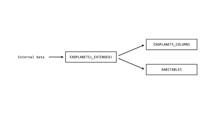
sqlite> SELECT * FROM HABITABLES LIMIT 5;So, we know that HABITABLES depends on the values in EXOPLANETS (or, equally, EXOPLANETS_EXTENDED), and EXOPLANETS_COLUMNS does as well. A dependency graph of our database looks like this:
Very simple lineage information, but already useful. Let’s look at an anomaly in HABITABLES in the context of this graph, and see what we can learn.
Investigating an anomaly
When we have a key metric, like habitability in HABITABLES, we can assess the health of that metric in several ways. For a start, what is the average value of habitability for new data on a given day?
Looking at this data, we see that something is wrong. The average value for habitability is normally around 0.5, but it halves to around 0.25 later in the recorded data.
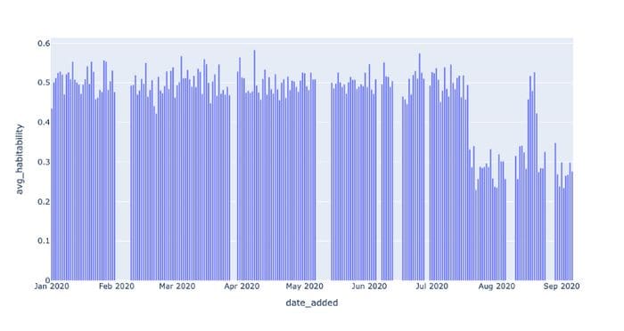
This is a clear distributional anomaly, but what exactly is going on? In other words, what is the root cause of this anomaly?
Why don’t we look at the NULL rate for habitability, like we did in Part I?
Fortunately, nothing looks out of character here:
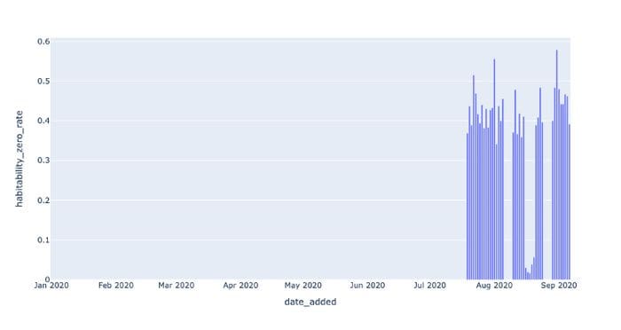
But this doesn’t look promising as the cause of our issue. What if we looked at another distributional health metric, the rate of zero values?
Something seems evidently more amiss here:
Historically, habitability was virtually never zero, but at later dates it spikes up to nearly 40% on average. This has the detected effect of lowering the field’s average value.
We can adapt one of the distribution detectors we built in Part I to get the first date of appreciable zero rates in the habitability field:
I ran this query through the command line:
$ sqlite3 EXOPLANETS.db < queries/lineage/habitability-zero-rate-detector.sql
DATE_ADDED | HABITABILITY_ZERO_RATE | PREV_HABITABILITY_ZERO_RATE
2020–07–19 | 0.369047619047619      | 0.0
2020–07–19 was the first date the zero rate began showing anomalous results. Recall that this is the same day as the schema change detection in EXOPLANETS_EXTENDED. EXOPLANETS_EXTENDED is upstream from HABITABLES, so it’s very possible that these two incidents are related.
It is in this way that lineage information can help us identify the root cause of incidents, and move quicker towards resolving them. Compare the two following explanations for this incident in HABITABLES:
- On 2020–07–19, the zero rate of the habitability column in the
HABITABLEStable jumped from 0% to 37%. - On 2020–07–19, we began tracking two additional fields,
eccentricityandatmosphere, in theEXOPLANETStable. This had an adverse effect on the downstream tableHABITABLES, often setting the fieldsmin_tempandmax_tempto extreme values whenevereccentricitywas notNULL. In turn, this caused thehabitabilityfield spike in zero rate, which we detected as an anomalous decrease in the average value.
Explanation (1) uses just the fact that an anomaly took place. Explanation (2) uses lineage, in terms of dependencies between both tables and fields, to put the incident in context and determine the root cause. Everything in (2) is actually correct, by the way, and I encourage you to mess around with the environment to understand for yourself what’s going on. While these are just simple examples, an engineer equipped with (2) would be faster to understand and resolve the underlying issue, and this is all owed to proper observability.
What’s next?
Tracking schema changes and lineage can give you unprecedented visibility into the health and usage patterns of your data, providing vital contextual information about who, what, where, why, and how your data was used. In fact, schema and lineage are the two most important data observability pillars when it comes to understanding the downstream (and often real-world) implications of data downtime.
To summarize:
- Observing our data’s schema means understanding the formal structure of our data, and when and how it changes.
- Observing our data’s lineage means understanding the upstream and downstream dependencies in our pipeline, and putting isolated incidents in a larger context.
- Both of these pillars of data observability involve tracking the proper metadata, and transforming our data in a way that makes anomalies understandable.
- Better observability means better understanding of why and how data breaks, reducing both time-to-detection and time-to-resolution.
We hope that this second installment of “Data Observability in Context” was useful.
Until Part III, here’s wishing you no data downtime!
Interested in learning more about Monte Carlo’s approach to data observability? Reach out to Ryan, Barr, and the Monte Carlo team.
Barr Moses is the CEO and Co-founder of Monte Carlo, a data observability company. Prior, she served as a VP of Operations at Gainsight.
Ryan Kearns is a data and machine learning engineer at Monte Carlo and a rising senior at Stanford University.
Original. Reposted with permission.
Related:
- Data Observability: Building Data Quality Monitors Using SQL
- Data Catalogs Are Dead; Long Live Data Discovery
- Data Cleaning and Wrangling in SQL