Deep Learning Recommendation Models (DLRM): A Deep Dive

By Nishant Kumar, Data Science Professional.

Recommendation systems are built to predict what users might like, especially when there are lots of choices available.

The DLRM algorithm was open-sourced by Facebook on March 31, 2019, and is part of the popular MLPerf Benchmark.

Deep Learning Recommendation Model Architecture (DLRM)

Why should you consider using DLRM?

This paper attempts to combine 2 important concepts that are driving the architectural changes in recommendation systems:

1. From the view of Recommendation Systems, initially, content filtering systems were employed that matched users to products based on their preferences. This subsequently evolved to use collaborative filtering where recommendations were based on past user behaviors.
2. From the view of Predictive Analytics, it relies on statistical models to classify or predict the probability of events based on the given data. These models shifted from simple models such as linear and logistic regression to models that incorporate deep networks.

In this paper, the authors claim to succeed in unifying these 2 perspectives in the DLRM Model.

A few notable features:

1. Extensive use of Embedding Tables: Embedding provides a rich and meaningful representation of the data of the users.
2. Exploits Multi-layer Perceptron (MLP): MLP presents a flavor of Deep Learning. They can well address the limitations presented by the statistical methods.
3. Model Parallelism: Poses less overhead on memory and speeds it up.
4. Interaction between Embeddings: Used to interpret latent factors (i.e., hidden factors) between feature interactions. An example would be how likely a user who likes comedy and horror movies would like a horror-comedy movie. Such interactions play a major role in the working of recommendation systems.

LET'S START

 

Model Workflow:

 

DLRM Workflow.

• The model uses embedding to process sparse features that represent categorical data and a Multi-layer Perceptron (MLP) to process dense features,
• Interacts these features explicitly using the statistical techniques proposed.
• Finally, it finds the event probability by post-processing the interactions with another MLP.

 

ARCHITECTURE:

 

1. Embeddings
2. Matrix Factorization
3. Factorization Machine
4. Multi-layer Perceptron (MLP)

Let’s discuss them in a little detail.

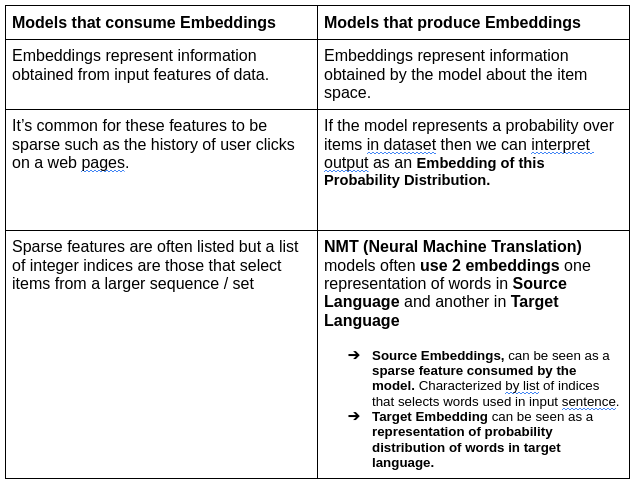
1. Embeddings

Mapping of concepts, objects, or items into a vector space is called an Embedding

E.g.,

In the context of neural networks, embeddings are low-dimensional, learned continuous vector representation of discrete variables.

Why should we use Embeddings instead of other options such as lists of sparse items?

• Reduces dimensionality of categorical variables and meaningfully represent categories in the abstract space.
• We can measure the distance between embeddings in a more meaningful way.
• Embedding elements represent sparse features in some abstract space relevant to the model at hand, while integers represent an ordering of the input data.
• Embedding vectors project n-dimensional items space into d-dimensional embedding vectors where n >> d.

2. Matrix Factorization

This technique belongs to a class of Collaborative filtering algorithms used in Recommendation Systems.

Matrix Factorization algorithms work by decomposing user-item interaction matrix into the product of 2 lower dimensionality rectangular matrices.

Refer to https://developers.google.com/machine-learning/recommendation/collaborative/matrix for more details.

3. Factorization Machines (FM)

A good choice for tasks dealing with high-dimensional sparse datasets.

FM is an improved version of MF. It is designed to capture interactions between features within high-dimensional sparse datasets economically.

Factorization Matrix (FM) Equation.

Features of Factorization Machines:

• Able to estimate interactions in sparse settings because they break the independence of interaction by parameters by factoring them.
• Incorporates second-order interactions into a linear model with categorical data by defining a model of the form,

FMs factorize second-order interaction matrix to its latent factors (or embedding vectors) as in matrix factorization, which more effectively handles sparse data.

Different orders of interaction matrices.

Significantly reduces the complexity of second-order interactions by only capturing interactions between pairs of distinct embedding vectors, yielding linear computational complexity.

Refer to https://docs.aws.amazon.com/sagemaker/latest/dg/fact-machines.html.

4. Multi-layer Perceptron

Finally, a little flavor of Deep Learning.

A Multi-layer Perceptron (MLP) is a class of Feed-Forward Artificial Neural Network.

An MLP consists of at least 3 layers of nodes:

• Input layer
• Hidden layer
• Output layer

Except for input nodes, each node is a neuron that uses a nonlinear activation function.

MLP utilizes supervised learning called Backpropagation for training.

These methods have been used to capture more complex interactions.

MLPs with sufficient depth and width can fit data to arbitrary precision.

One specific case, Neural Collaborative Filtering (NCF), used as part of MLPerf Benchmark, uses an MLP rather than dot product to compute interactions between embeddings in Matrix Factorization.

 

DLRM Operators by Framework

 

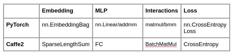
You can find below the overall architecture of open-source recommendation model system. All configurable parameters are outlined in blue. And the operators used are shown in green.

Source: https://arxiv.org/pdf/1906.03109.pdf.

We have 3 tested models from Facebook (Source: Architectural Implication of Facebook’s DNN-Based Personalized Recommendation)

Model Architecture parameters are representative of production scale recommendation workloads for 3 examples of recommendation models used, highlighting their diversity in terms of embedding table and FC sizes. Each parameter (column) is normalized to the smallest instance across all 3 configurations.

 

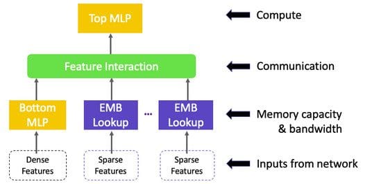
ISSUES

 

1. Memory Capacity Dominated (Input from Network)
2. Memory Band-Width Dominated (Processing of Features: Embedding Lookup and MLP)
3. Communication Based (Interaction between Features)
4. Compute Dominated (Compute/Run-Time Bottleneck)

 

1. Memory Capacity Dominated

 

(Input From Network)

Source: https://arxiv.org/pdf/1906.00091.pdf.

SOLUTION: Parallelism

One of the basic and most important steps

• Embeddings contribute the majority of parameters, with several tables each requiring an excess of multiple GBs of memory. This necessitates the distribution of models across multiple devices.
• MLP parameters are smaller in memory but translate to sizeable amounts of compute

Data Parallelism is preferred for MLPs since this enables concurrent processing of samples on different devices and only requires communication when accumulating updates.

Personalization:

SETUP: Top MLP and interaction operator requires access to part of mini-batch from the bottom MLP and all of the embeddings. Since model parallelism has been used to distribute embeddings across devices, this requires a personalized all-to-all communication.

Butterfly Shuffle for the all-to-all (Personalized) Communication. Source: https://arxiv.org/pdf/1906.00091.pdf.

Slices (i.e., 1,2,3) are Embedding vectors that are supposed to be transferred to target devices for personalization.

Currently, transfers are only explicit copies.

 

2. Memory Bandwidth Dominated

 

(Processing of Features: Embedding Lookup and MLP)

Source: https://arxiv.org/pdf/1909.02107.pdf, https://arxiv.org/pdf/1901.02103.pdf.

• MLP parameters are smaller in memory but translate to sizeable amounts of compute (so the issue will come during compute).
• Embedding lookups can cause memory constraints.

SOLUTION: Compositional Embeddings using Complementary Partitions

Representation of n items in d dimensional vector space can be broadly divided into 2 categories:

An approach is proposed for generating unique embedding for each categorical feature using Complementary Partitions of category set to generate Compositional Embeddings.

Approaching Memory-Bandwidth Consumption issue:

1. Hashing Trick
2. Quotient-Remainder Trick

HASHING TRICK:

Naive approach of reducing embedding table using a simple hash function.

Hashing Trick.

It significantly reduces the size of the embedding matrix from O(|S|D) to O(mD) since m << |S|.

Disadvantages -

• Does not yield a Unique Embedding for each Category.
• Naively maps multiple categories to the same embedding vector.
• Results in loss of Information,hence, rapid deterioration of model quality.

QUOTIENT-REMAINDER TRICK:

Using 2 complementary functions, i.e., integer quotient and remainder functions: we can produce 2 separate embedding tables and combine them in a way that yields a unique embedding for each category.

It results in memory complexity O(D*|S|/m + mD), a slight increase in memory compared to hashing trick,

• But with an added benefit of producing a unique representation.

Quotient-Remainder Trick.

Complementary Partitions

In the Quotient-Remainder trick, each operation partitions a set of categories in to “Multiple Buckets” such that every index in the same “bucket” is mapped to the same vector.

By combining embeddings from both quotient and remainder together, one is able to generate a distinct vector for each index.

NOTE: Complementary Partitions: Avoids repetition of data or embedding tables across partitions (as it’s complementary, duh!! )

Types Based on structure:

• Naive Complementary Partition
• Quotient — Remainder Complementary Partitions
• Generalized Quotient-Remainder Complementary Partitions
• Chinese Remainder Partitions

Types Based on Function:

Types of Complementary Partitions based on function.

Operation Based Compositional Embeddings:

Assume that vectors in each embedding table are distinct. If concatenation operation is used, then compositional embeddings of any category are unique.

This approach reduces the memory complexity of storing the entire embedding table O(|S|D) to O(|P1|D1+|P2|D2+…|Pk|Dk).

Operation-based embeddings are more complex due to the operations applied.

Path Based Compositional Embeddings:

Each function in a composition is determined based on a unique set of equivalence classes from each partition, yielding a unique ‘path’ of transformations.

Path Based Compositional Embeddings are expected to give better results with the benefit of lower model complexity.

TRADE-OFF - 

There’s a catch.

• A larger embedding table will yield better model quality but at the cost of increased memory requirements.
• Using a more aggressive version will yield smaller models but lead to a reduction in model quality.
• Most models exponentially decrease in performance with a number of parameters.
• Both types of compositional embeddings reduce the number of parameters by implicitly enforcing some structure defined bycomplementary partitions in the generation of each category’s embedding.
• The quality of the model ought to depend on how closely the chosen partitions reflect intrinsic properties of the category set and their respective embeddings.

 

3. Communication Based

 

(Interaction between Features)

Source: https://github.com/thumbe3/Distributed_Training_of_DLRM/blob/master/CS744_group10.pdf.

DLRM uses model parallelism to avoid replicating the whole set of embedding tables on every GPU device and data parallelism to enable concurrent processing of samples in FC layers.

MLP parameters are replicated across GPU devices and not shuffled.

What is the problem?

Transferring embedding tables across nodes in a cluster becomes expensive and could be a Bottleneck.

Solution:

Since it is the interaction between pairs of learned embedding vectors that matters and not the absolute values of embedding themselves.

We hypothesize we can learn embeddings in different nodes independently to result in a good model.

Saves Network Bandwidth by synchronizing only MLP parameters and learning Embedding tables independently on each of the server nodes.

In order to speed up training, sharding of input dataset across cluster nodes has been implemented such that both nodes can process different shards of data concurrently and therefore make more progress than a single node.

Distributed DLRM.

Master node collects gradients of MLP parameters from the slave node and itself. MLP parameters were synchronized by monitoring their values for some of the experiments.

Embedding tables learned were different in both nodes as these are not synchronized, and nodes work on different shards of the input dataset.

Since the DLRM uses Interaction of Embeddings rather than embedding themselves, good models were achievable even though embeddings were not synchronized across the nodes.

 

4. Compute Dominated

 

(Compute/Run-Time Bottleneck)

Source: https://github.com/pytorch/FBGEMM/wiki/Recent-feature-additions-and-improvements-in-FBGEMM, https://engineering.fb.com/ml-applications/fbgemm/

As discussed above,

• MLP also results in Compute Overload
• Co-location creates performance bottlenecks when running production-scale recommendation models leading to lower resource utilization

Co-location impacts more on SparseLengthSum due to higher irregular memory accesses, which exhibits less cache reuse.

SOLUTION: FBGEMM (Facebook + General Matrix Multiplication)

Introducing the workhorse of our model

It is the definite back-end of PyTorch for quantized inference on servers.

• It is specifically optimized for low-precision data, unlike the conventional linear algebra libraries used in scientific computing (which work with FP32 or FP64 precision).
• It provides efficient low-precision general matrix-matrix multiplication (GEMM) for small batch sizes and support for accuracy-loss-minimizing techniques such as row-wise quantization and outlier-aware quantization.
• It also exploits fusion opportunities to overcome the unique challenges of matrix multiplication at lower precision with bandwidth-bound pre- and post-GEMM operations.

A number of improvements to the existing features as well as new features were added in the January 2020 release.

These include Embedding Kernels (very important to us) JIT’ed sparse kernels and int64 GEMM for Privacy Preserving Machine Learning Models.

A couple of implementation stats:

1. Reduces DRAM bandwidth usage in Recommendation Systems by 40%
2. Speeds up character detection by 2.4x in Rosetta(ML Algo for detecting text in Images and Videos)

Computations occur on 64-bit Matrix Multiplication Operations, which is widely used in Privacy Preserving field, essentially speeding up Privacy Preserving Machine Learning Models.

Currently, there exists no good high-performance implementation of 64-bit GEMMs on the current generation of CPUs.

Therefore, 64-bit GEMMs have been added to FBGEMM. It achieves 10.5 GOPs/sec on Intel Xeon Gold 6138 processor with turbo off. It is 3.5x faster than the existing implementation that runs at 3 GOps/sec. This is the first iteration of the 64-bit GEMM implementation.

 

REFERENCES

 

1. Recommendation series by James Le: It’s really good for building up basics on Recommendation Systems. https://jameskle.com/writes/rec-sys-part-1
2. Deep Learning Recommendation Model for Personalization and Recommendation Systems https://arxiv.org/pdf/1906.00091.pdf
3. Compositional Embeddings Using Complementary Partitionsfor Memory-Efficient Recommendation Systems https://arxiv.org/pdf/1909.02107.pdf
4. On the Dimensionality of Embeddings for Sparse Features and Data https://arxiv.org/pdf/1901.02103.pdf
5. The Architectural Implications of Facebook’s DNN-based Personalized Recommendation https://arxiv.org/pdf/1906.03109.pdf
6. https://github.com/pytorch/FBGEMM/wiki/Recent-feature-additions-and-improvements-in-FBGEMM
7. Open-sourcing FBGEMM for state-of-the-art server-side inference https://engineering.fb.com/ml-applications/fbgemm/

 

Original. Reposted with permission.

 

Bio: Nishant Kumar holds a Bachelor's Degree in Computer Science. He has over 4 years of IT industry experience in various domains related to Data Science including Machine Learning, NLP, Recommendation Systems. When he is not playing around with data he spends time Cycling, and cooking. He loves to write technical articles on technical aspects of Data Science and interesting Research in NLP. You can check out articles on Medium.

Related:

• Algorithms of Social Manipulation
• How LinkedIn Uses Machine Learning in its Recruiter Recommendation Systems
• Content-Based Recommendation System using Word Embeddings