High-Performance Deep Learning: How to train smaller, faster, and better models – Part 3

In the previous parts (Part 1 & Part 2), we discussed why efficiency is important for deep learning models to achieve high-performance models that are pareto-optimal, as well as the focus areas for efficiency in Deep Learning. Let us now dive deeper into examples of tools and techniques that fall in these focus areas.

 

Compression Techniques

 

Compression techniques, as mentioned earlier, are generic techniques that can help achieve a more efficient representation of one or more layers in a neural network, with a possible quality trade-off. The efficiency could come from improving one or more of the footprint metrics, such as model size, inference latency, training time required for convergence, etc., in exchange for as little quality loss as possible. Often the model could be over-parameterized. In such cases, these techniques help improve generalization on unseen data as well.

Pruning: One of the popular compression techniques is Pruning, where we prune unimportant network connections, hence making the network sparse. LeCun et al. [1], in their paper titled "Optimal Brain Damage", trimmed the number of parameters (connections between layers) in their neural network by a factor of four while increasing both the inference speed and generalization.

An illustration of pruning in neural networks.

A similar approach was followed by the Optimal Brain Surgeon work (OBD) by Hassibi et al. [2] and by Zhu et al. [3]. These methods take a network that has been pre-trained to reasonable quality and then iteratively prune the parameters that have the lowest saliency score, which measures the importance of a particular connection, such that the impact on the validation loss is minimized. Once pruning concludes, the network is fine-tuned with the remaining parameters. The process is repeated until the network is pruned to the desired level.

Amongst the various works on pruning, the differences occur in the following dimensions:

• Saliency: This is the heuristic for determining which connection should be pruned. This can be based on second-order derivatives [1, 2] of the connection weight with respect to the loss function, the magnitude of the connection weight [3], and so on.
• Unstructured v/s Structured: The most flexible way of pruning is unstructured (or random) pruning, where all given parameters are treated equally. In structured pruning, parameters are pruned in blocks of size > 1 (such as pruning row-wise in a weight matrix or pruning channelwise in a convolutional filter (example: [4,5]). Structured pruning allows easier leveraging of inference-time gains in size and latency since these blocks of pruned parameters can be intelligently skipped for storage and inference.

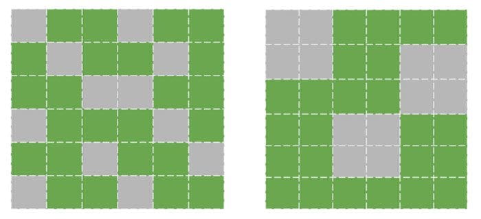
Unstructured vs. Structured Pruning of a weight matrix, respectively.

• Distribution: One could set a pruning budget that is the same for each layer, or it could be allocated on a per-layer basis [6]. The intuition being that certain layers are more amenable to pruning than others. For example, often, the first few layers are already small enough that they cannot tolerate significant sparsity [7].
• Scheduling: Yet additional criteria are how much to prune and when? Do we want to prune an equal number of parameters every round [8], or do we prune at a higher pace in the beginning and gradually slow down [9]?
• Regrowth: In some cases, the network is allowed to regrow the pruned connections [9], such that the network constantly operates with the same percentage of connections pruned.

In terms of practical usage, structured pruning with a meaningful block size can help improve latency. Elsen et al. [7] construct sparse convolutional networks that outperform their dense counterparts by 1.3 - 2.4× with ≈ 66% of the parameters while retaining the same Top-1 accuracy. They do this via their library to convert from the NHWC (channels-last) standard dense representation to a special NCHW (channels-first) ‘Block Compressed Sparse Row’ (BCSR) representation which is suitable for fast inference using their fast kernels on ARM devices, WebAssembly etc. [10]. Although they also introduce some constraints on the kinds of sparse networks that can be accelerated. Overall, this is a promising step towards practical improvements in footprint metrics with pruned networks.

Quantization:  Quantization is another popular compression technique. It exploits the idea that almost all the weights of a typical network are in 32-bit floating-point values, and if we are okay with losing some model quality (accuracy, precision, recall, etc.), we can store these values in a lower precision format (16-bit, 8-bit, 4-bit, etc.).

For example, when a model is persisted, we can map the minimum value in a weight matrix to 0 and the maximum value to 2^b-1 (where b is the number of bits of precision), and linearly extrapolate all values between them to an integer value. Often, this might be sufficient for the purposes of reducing model size. For example, if b = 8, we are mapping the 32-bit floating-point weights to 8-bit unsigned integers. This would lead to a 4x reduction in space. When doing inference (computing model predictions), we can recover a lossy representation of the original floating-point value (due to the rounding error), using the quantized value and the min & max floating-point values of the array. This step is referred to as Weight Quantization since we are quantizing the model’s weights.

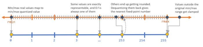
Mapping continuous high-precision values to discrete low-precision integer values. Source

The lossy representation and the rounding error might be okay for larger networks with built-in redundancy due to a large number of parameters but might lead to a drop in accuracy for smaller networks, which would likely be sensitive to these errors.

We can solve this issue (in an experimental manner) by simulating the rounding behavior of weight quantization during the training. We do this by adding nodes in the model training graph that quantize and dequantize the activations and weight matrices, such that the training-time inputs to a neural network operation look identical to what they would have during the inference stage. Such nodes are referred to as Fake Quantization nodes. Training in such a manner makes the networks more robust to the behavior of quantization in inference mode. Note that we are doing Activation Quantization along with Weight Quantization during training now. This step of training-time simulated quantization is described in detail by Jacob et al. and Krishnamoorthi et al. [11,12]

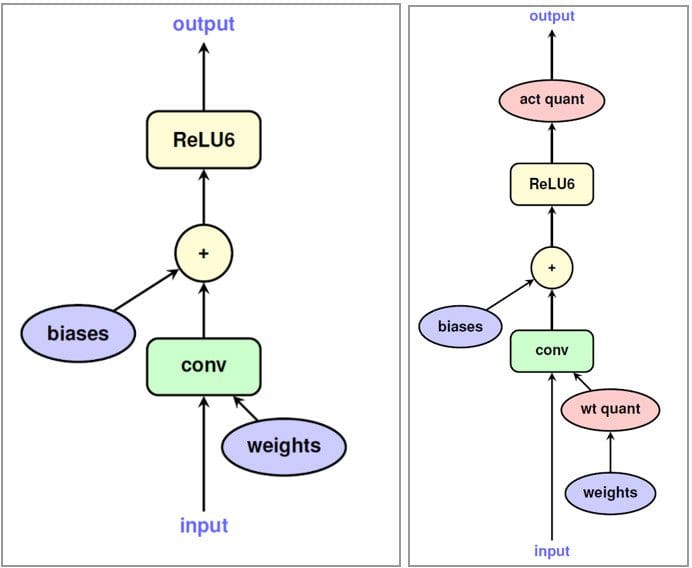
Original model training graph and the graph with fake quantization nodes. Source

Since both weights and activations are run in simulated quantized mode, that means all layers receive inputs that could be represented in lower-precision, and after the model is trained, it should be robust enough to do the math operations directly in lower-precision. As an example, if we train the model to replicate quantization in the 8-bit domain, the model can be deployed to do the matrix multiplication and other operations with 8-bit integers.

On resource-constrained devices (such as mobile, embedded, and IoT devices), 8-bit operations can be sped up between 1.5 - 2x using libraries like GEMMLOWP [13] which rely on hardware support for such acceleration such as the Neon intrinsics on ARM processors [14]. Further, frameworks such as Tensorflow Lite enable their users to directly use quantized operations without having to bother about the lower-level implementations.

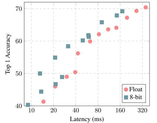
Top-1 Accuracy vs. Model Latency for models with and without quantization. Source

Apart from Pruning and Quantization, there are other techniques like Low-Rank Matrix Factorization, K-Means Clustering, Weight-Sharing etc. which are also actively being used for model compression [15].

Overall, we saw that compression techniques could be used to reduce a model’s footprint (size, latency, etc.) while trading off some quality (accuracy, precision, recall, etc.) in return.

 

Learning Techniques

 

Distillation: As mentioned earlier, Learning techniques try to train a model differently in order to obtain a better performance. For example, Hinton et al. [16], in their seminal work, explored how smaller networks can be taught to extract dark knowledge from larger models/ensembles of larger models. They use a larger teacher model to generate soft labels on existing labeled data.

The soft labels assign a probability to each possible class instead of hard binary values in the original data. The intuition is that these soft labels capture the relationship between the different classes from which the model can learn. For example, a truck is more similar to a car than to an apple, which the model might not be able to learn directly from hard labels. The student network learns to minimize the cross-entropy loss on these soft labels, along with the original ground-truth hard labels. The weights of each of these loss functions can be scaled based on the results from experimentation.

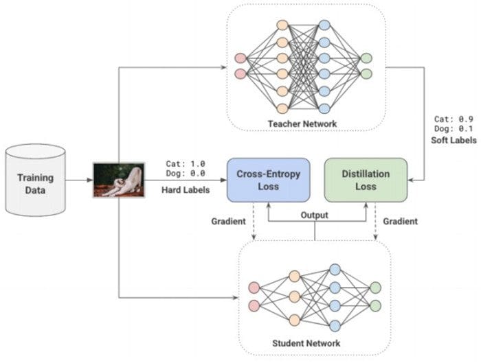
Distillation of a smaller student model from a larger pre-trained teacher model.

In the paper, Hinton et al. [16] were able to closely match the accuracy of a 10-model ensemble for a speech recognition task with a single distilled model. There are other comprehensive studies [17,18] demonstrating the significant improvements in model quality of smaller models. As an example, Sanh. et al. [18] were able to distill a student model that retains 97% of the performance of BERT-Base while being 40% smaller and 60% faster on CPU.

Data Augmentation: Typically for large models and complex tasks, the more data you have, the higher the chances of improving your model’s performance. However, getting high-quality labeled data is often both slow and expensive since they usually require a human in the loop. Learning from this data which has been labeled by humans, is referred to as supervised learning. It works very well when we have the resources to pay for the labels, but we can and should do better.

Data Augmentation is a nifty way of improving the performance of the model. Usually, it involves making transformations to your data, such that it does not require re-labeling (label-invariant transformations). For example, if you were teaching your neural network to classify an image to contain a dog or a cat, rotating the image would not change the label. Other transformations could be horizontal/vertical flipping, stretching, cropping, adding Gaussian noise, etc. Similarly, if you were detecting the sentiment of a given piece of text, introducing a typo would likely not change the label.

Such label-invariant transformations have been used across the board in popular deep learning models. They are especially handy when you have a large number of classes and/or few examples for certain classes.

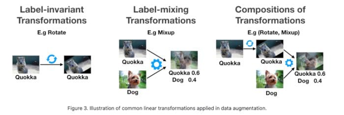
Some common types of data augmentations. Source

There are other transformations such as Mixup [19], which mix inputs from two different classes in a weighted manner and treat the label to be a similarly weighted combination of the two classes. The idea is that the model should be able to extract out features that are relevant for both classes.

These techniques are really introducing data efficiency to the pipeline. It is not very different from teaching a kid to identify real-life objects in different contexts.

Self-Supervised Learning: There is rapid progress in an adjacent area, where we can learn generic models that completely skip the need for labels for extracting meaning out of data. With methods like contrastive learning [20], we can train a model such that it learns a representation for the input, such that similar inputs would have similar representations, while unrelated inputs should have very dissimilar representations. These representations are n-dimensional vectors (embeddings) which can then be useful as features in other tasks where we might not have enough data to train models from scratch. We can view the first step of using unlabeled data as pre-training and the next step as fine-tuning.

Contrastive Learning. Source

This two-step process of pre-training on unlabeled data and fine-tuning on labeled data has also gained rapid acceptance in the NLP community. ULMFiT [21] pioneered the idea of training a general-purpose language model, where the model learns to solve the task of predicting the next word in a given sentence.

The authors found that using a large corpus of preprocessed but unlabeled data such as the WikiText-103 (derived from English Wikipedia pages) was a good choice for the pre-training step. This was sufficient for the model to learn general properties about the language. The authors found that fine-tuning such a pre-trained model for a binary classification problem required only 100 labeled examples (as compared to 10,000 labeled examples otherwise).

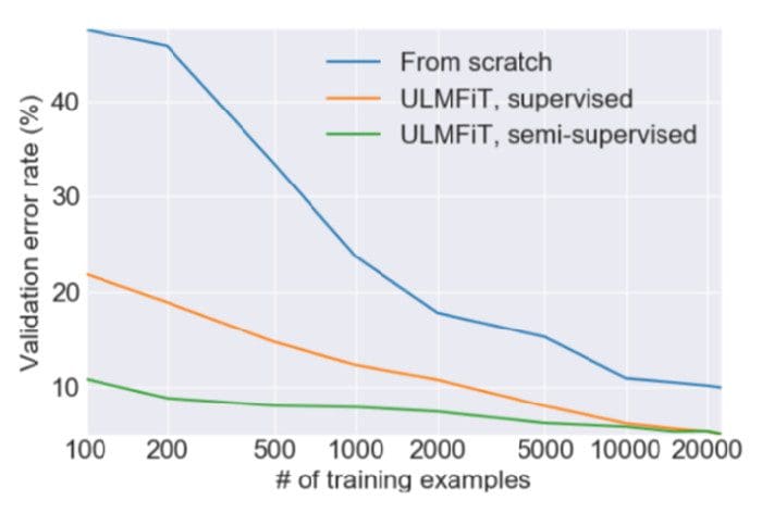
Rapid convergence with ULMFiT. Source

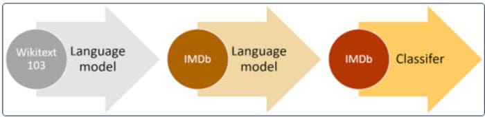
High-level approach of pre-training on a large corpus and fine-tuning on the relevant dataset. Source

This idea was also explored in BERT models, where the pre-training steps involve learning a  bi-directional masked language model, such that the model has to predict a missing word in the middle of a sentence.

Overall, learning techniques help us improve model quality without impacting the footprint. This could be used for improving model quality for deployment. If the original model quality was satisfactory, you could also exchange the newfound quality gains for improving model size and latency by simply reducing the number of parameters in your network until you go back to the minimum viable model quality.

In our next part, we will continue to go over examples of tools and techniques that fit in the remaining three focus areas. Also, feel free to go over our survey paper that explores this topic in detail.

 

References

[1] Yann LeCun, John S Denker, and Sara A Solla. 1990. Optimal brain damage. In Advances in neural information processing systems. 598–605.

[2] Babak Hassibi, David G Stork, and Gregory J Wolff. 1993. Optimal brain surgeon and general network pruning. In IEEE international conference on neural networks. IEEE, 293–299.

[3] Michael Zhu and Suyog Gupta. 2018. To Prune, or Not to Prune: Exploring the Efficacy of Pruning for Model Compression. In 6th International Conference on Learning Representations, ICLR 2018, Vancouver, BC, Canada, April 30 - May 3, 2018, Workshop Track Proceedings. OpenReview.net. https://openreview.net/forum?id=Sy1iIDkPM

[4] Sajid Anwar, Kyuyeon Hwang, and Wonyong Sung. 2017. Structured pruning of deep convolutional neural networks. ACM Journal on Emerging Technologies in Computing Systems (JETC) 13, 3 (2017), 1–18.

[5] Hao Li, Asim Kadav, Igor Durdanovic, Hanan Samet, and Hans Peter Graf. 2016. Pruning Filters for Efficient ConvNets. In ICLR (Poster).

[6] Xin Dong, Shangyu Chen, and Sinno Jialin Pan. 2017. Learning to prune deep neural networks via layer-wise optimal brain surgeon. arXiv preprint arXiv:1705.07565 (2017).

[7] Erich Elsen, Marat Dukhan, Trevor Gale, and Karen Simonyan. 2020. Fast sparse convnets. In Proceedings of the IEEE/CVF conference on computer vision and pattern recognition. 14629–14638.

[8] Song Han, Jeff Pool, John Tran, and William J Dally. 2015. Learning both weights and connections for efficient neural networks. arXiv preprint arXiv:1506.02626 (2015).

[9] Tim Dettmers and Luke Zettlemoyer. 2019. Sparse networks from scratch: Faster training without losing performance. arXiv preprint arXiv:1907.04840 (2019).

[10] XNNPACK. https://github.com/google/XNNPACK

[11] Benoit Jacob, Skirmantas Kligys, Bo Chen, Menglong Zhu, Matthew Tang, Andrew Howard, Hartwig Adam, and Dmitry Kalenichenko. 2018. Quantization and training of neural networks for efficient integer-arithmetic-only inference. In Proceedings of the IEEE Conference on Computer Vision and Pattern Recognition. 2704–2713

[12] Raghuraman Krishnamoorthi. 2018. Quantizing deep convolutional networks for efficient inference: A whitepaper. arXiv (Jun 2018). arXiv:1806.08342 https://arxiv.org/abs/1806.08342v1

[13] GEMMLOWP. https://github.com/google/gemmlowp

[14] Arm Ltd. 2021. SIMD ISAs | Neon – Arm Developer. https://developer.arm.com/architectures/instruction-sets/simdisas/neon [Online; accessed 3. Jun. 2021].

[15] Rina Panigrahy. 2021. Matrix Compression Operator. https://blog.tensorflow.org/2020/02/matrix-compressionoperator-tensorflow.html

[16] Geoffrey Hinton, Oriol Vinyals, and Jeff Dean. 2015. Distilling the knowledge in a neural network. arXiv preprint arXiv:1503.02531 (2015).

[17] Gregor Urban, Krzysztof J Geras, Samira Ebrahimi Kahou, Ozlem Aslan, Shengjie Wang, Rich Caruana, Abdelrahman Mohamed, Matthai Philipose, and Matt Richardson. 2016. Do deep convolutional nets really need to be deep and convolutional? arXiv preprint arXiv:1603.05691 (2016).

[18] Victor Sanh, Lysandre Debut, Julien Chaumond, and Thomas Wolf. 2019. DistilBERT, a distilled version of BERT: smaller, faster, cheaper and lighter. arXiv preprint arXiv:1910.01108 (2019).

[19] Hongyi Zhang, Moustapha Cisse, Yann N Dauphin, and David Lopez-Paz. 2017. mixup: Beyond empirical risk minimization. arXiv preprint arXiv:1710.09412 (2017).

[20] Ting Chen, Simon Kornblith, Mohammad Norouzi, and Geoffrey Hinton. 2020. A simple framework for contrastive learning of visual representations. In International conference on machine learning. PMLR, 1597–1607.

[21] Jeremy Howard and Sebastian Ruder. 2018. Universal language model fine-tuning for text classification. arXiv preprint arXiv:1801.06146 (2018).

Bio: Gaurav Menghani is a Staff Software Engineer at Google Research where he leads research projects geared towards optimizing large machine learning models for efficient training and inference on devices ranging from tiny microcontrollers to Tensor Processing Unit (TPU)-based servers. His work has positively impacted > 1 Billion of active users across YouTube, Cloud, Ads, Chrome, etc. He is also an author of an upcoming book with Manning Publication on Efficient Machine Learning. Before Google, Gaurav worked at Facebook for 4.5 years and has contributed significantly to Facebook’s Search system and large-scale distributed databases. He has an M.S. in Computer Science from Stony Brook University.

twitter.com/GauravML
linkedin.com/in/gauravmenghani
www.gaurav.im

Related:

• High Performance Deep Learning, Part 1
• High-Performance Deep Learning: How to train smaller, faster, and better models – Part 2
• 5 Challenges to Scaling Machine Learning Models