How to Determine the Best Fitting Data Distribution Using Python
Approaches to data sampling, modeling, and analysis can vary based on the distribution of your data, and so determining the best fit theoretical distribution can be an essential step in your data exploration process.
Sometimes you know the best fitting distribution, or probability density function, of your data prior to analysis; more often, you do not. Approaches to data sampling, modeling, and analysis can vary based on the distribution of your data, and so determining the best fit theoretical distribution can be an essential step in your data exploration process.
This is where distfit comes in.
distfitis a python package for probability density fitting across 89 univariate distributions to non-censored data by residual sum of squares (RSS), and hypothesis testing. Probability density fitting is the fitting of a probability distribution to a series of data concerning the repeated measurement of a variable phenomenon.distfitscores each of the 89 different distributions for the fit with the empirical distribution and return the best scoring distribution.
Essentially, we can pass our data to distfit and have it determine which probability distribution the data best fits, based on an RSS metric, after it attempts to fit the data to 89 different distributions. We can then view a visualization overlay of the empirical data and the best fit distribution. We can also view a summary of the process, as well as plot the best-fit results.
Let's have a look at how to use distfit to accomplish these tasks, and see just how simple it is to use.
First, we will generate some data; initialize the distfit model; and fit the data to the model. This is the core of the distfit distribution fitting process.
import numpy as np
from distfit import distfit

# Generate 10000 normal distribution samples with mean 0, std dev of 3
X = np.random.normal(0, 3, 10000)

# Initialize distfit
dist = distfit()

# Determine best-fitting probability distribution for data
dist.fit_transform(X)
And distfit toils away:
[distfit] >fit..
[distfit] >transform..
[distfit] >[norm      ] [0.00 sec] [RSS: 0.0004974] [loc=-0.002 scale=3.003]
[distfit] >[expon     ] [0.00 sec] [RSS: 0.1595665] [loc=-12.659 scale=12.657]
[distfit] >[pareto    ] [0.99 sec] [RSS: 0.1550162] [loc=-7033448.845 scale=7033436.186]
[distfit] >[dweibull  ] [0.28 sec] [RSS: 0.0027705] [loc=-0.001 scale=2.570]
[distfit] >[t         ] [0.25 sec] [RSS: 0.0004996] [loc=-0.002 scale=2.994]
[distfit] >[genextreme] [0.64 sec] [RSS: 0.0010127] [loc=-1.105 scale=3.007]
[distfit] >[gamma     ] [0.39 sec] [RSS: 0.0005046] [loc=-268.356 scale=0.034]
[distfit] >[lognorm   ] [0.84 sec] [RSS: 0.0005159] [loc=-227.504 scale=227.485]
[distfit] >[beta      ] [0.33 sec] [RSS: 0.0005016] [loc=-2746819.537 scale=2747059.862]
[distfit] >[uniform   ] [0.00 sec] [RSS: 0.1103102] [loc=-12.659 scale=22.811]
[distfit] >[loggamma  ] [0.73 sec] [RSS: 0.0005070] [loc=-554.304 scale=83.400]
[distfit] >Compute confidence interval [parametric]
Once complete, we can inspect the results in a few different ways. First, let's have a look at the summary that is generated.
# Print summary of evaluated distributions
print(dist.summary)
         distr        score  LLE          loc        scale  \
0         norm  0.000497419  NaN  -0.00231781      3.00297
1            t  0.000499624  NaN  -0.00210365      2.99368
2         beta  0.000501588  NaN -2.74682e+06  2.74706e+06
3        gamma  0.000504569  NaN     -268.356    0.0336241
4     loggamma  0.000506987  NaN     -554.304      83.3997
5      lognorm   0.00051591  NaN     -227.504      227.485
6   genextreme   0.00101271  NaN     -1.10495      3.00708
7     dweibull   0.00277053  NaN  -0.00114977      2.56974
8      uniform      0.11031  NaN      -12.659      22.8107
9       pareto     0.155016  NaN -7.03345e+06  7.03344e+06
10       expon     0.159567  NaN      -12.659      12.6567

                                       arg
0                                       ()
1                     (323.7785925192121,)
2   (73202573.87887828, 6404.720016859684)
3                     (7981.006169767873,)
4                     (770.4368441223046,)
5                  (0.013180038142300822,)
6                   (0.25551845624380576,)
7                    (1.2640245435189867,)
8                                       ()
9                     (524920.1083231748,)
10                                      ()
Based on the RSS (which is the 'score' in the above summary), and recalling that the lowest RSS will provide the best fit, our data best fits the normal distribution.
This may seem like a foregone conclusion, given that we sampled from the normal distribution, but that is not the case. Given the similarity between numerous distributions, consecutive runs on resampled data using the normal distribution show it is just as easy (perhaps easier?) to end up with a best fit distribution of t, gamma, beta, log-normal, or log-gamma, to name but a few, especially on relatively low sample sizes.
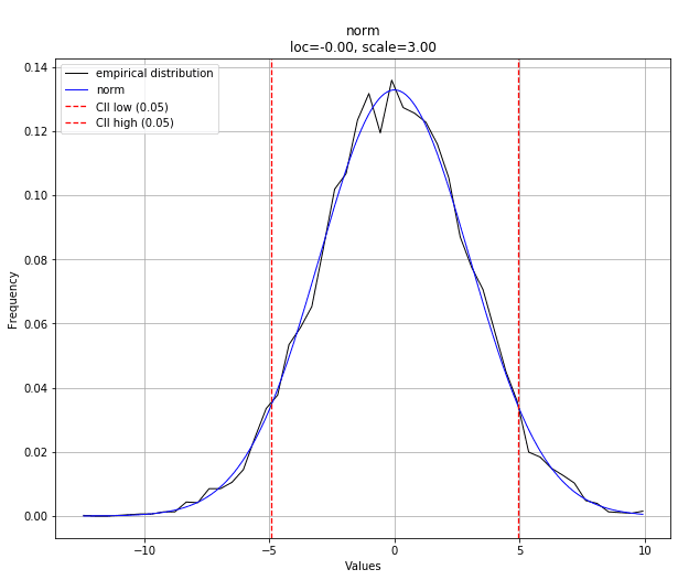
We can then plot the results of the best fit distribution against our empirical data.
# Plot results
dist.plot()
Finally, we can plot the best fit summary to see how the fit of distributions compare to one another, visually.
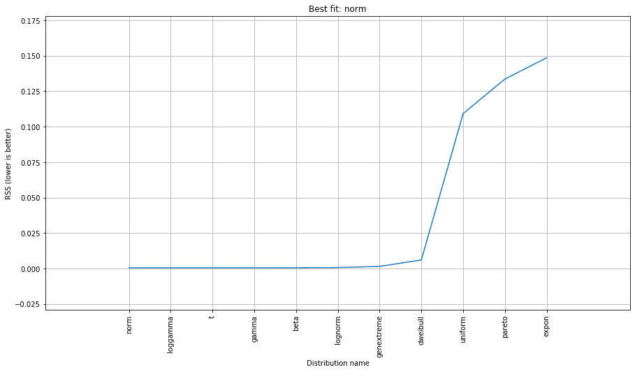
From the above, you can see relative goodness of fits of several of the best-fitting distributions to our data.
Besides the distribution fitting, distfit has other use cases as well:
The
distfitfunction has many use-cases. First of all to determine the best theoretical distribution for your data. This can reduce tens-of-thousands of data points into 3 floating parameters. Another application is for outlier detection. A null-distribution can be determined using the normal state. New datapoints that deviate significantly can then be marked as outliers, and are potentially of interest. The null-distribution can also be generated by randomization/permutation approaches. In such case, the new datapoints will be marked if it significantly deviates from randomness.
You can find examples for these use cases in the distfit documentation.
Matthew Mayo (@mattmayo13) is a Data Scientist and the Editor-in-Chief of KDnuggets, the seminal online Data Science and Machine Learning resource. His interests lie in natural language processing, algorithm design and optimization, unsupervised learning, neural networks, and automated approaches to machine learning. Matthew holds a Master's degree in computer science and a graduate diploma in data mining. He can be reached at editor1 at kdnuggets[dot]com.