An Introduction to Reinforcement Learning with OpenAI Gym, RLlib, and Google Colab
Get an Introduction to Reinforcement Learning by attempting to balance a virtual CartPole with OpenAI Gym, RLlib, and Google Colab.
By Michael Galarnyk & Sven Mika
This tutorial will use reinforcement learning (RL) to help balance a virtual CartPole. The video above from PilcoLearner shows the results of using RL in a real-life CartPole environment.
One possible definition of reinforcement learning (RL) is a computational approach to learning how to maximize the total sum of rewards when interacting with an environment. While a definition is useful, this tutorial aims to illustrate what reinforcement learning is through images, code, and video examples and along the way introduce reinforcement learning terms like agents and environments.
In particular, this tutorial explores:
- What is Reinforcement Learning
- The OpenAI Gym CartPole Environment
- The Role of Agents in Reinforcement Learning
- How to Train an Agent by using the Python Library RLlib
- How to use a GPU to Speed Up Training
- Hyperparameter Tuning with Ray Tune
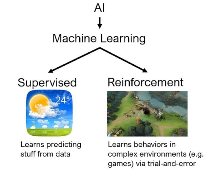
What is Reinforcement Learning
As a previous post noted, machine learning (ML), a sub-field of AI, uses neural networks or other types of mathematical models to learn how to interpret complex patterns. Two areas of ML that have recently become very popular due to their high level of maturity are supervised learning (SL), in which neural networks learn to make predictions based on large amounts of data, and reinforcement learning (RL), where the networks learn to make good action decisions in a trial-and-error fashion, using a simulator.
RL is the tech behind mind-boggling successes such as DeepMind’s AlphaGo Zero and the StarCraft II AI (AlphaStar) or OpenAI’s DOTA 2 AI (“OpenAI Five”). Note that there are many impressive uses of reinforcement learning and the reason why it is so powerful and promising for real-life decision making problems is because RL is capable of learning continuously — sometimes even in ever changing environments — starting with no knowledge of which decisions to make whatsoever (random behavior).
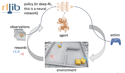
Agents and Environments
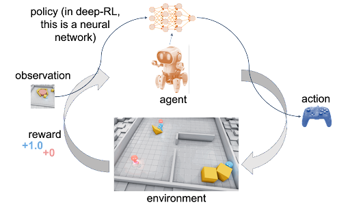
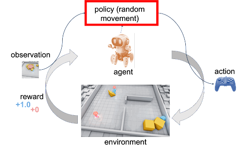
The diagram above shows the interactions and communications between an agent and an environment. In reinforcement learning, one or more agents interact within an environment which may be either a simulation like CartPole in this tutorial or a connection to real-world sensors and actuators. At each step, the agent receives an observation (i.e., the state of the environment), takes an action, and usually receives a reward (the frequency at which an agent receives a reward depends on a given task or problem). Agents learn from repeated trials, and a sequence of those is called an episode — the sequence of actions from an initial observation up to either a “success” or “failure” causing the environment to reach its “done” state. The learning portion of an RL framework trains a policy about which actions (i.e., sequential decisions) cause agents to maximize their long-term, cumulative rewards.
The OpenAI Gym Cartpole Environment
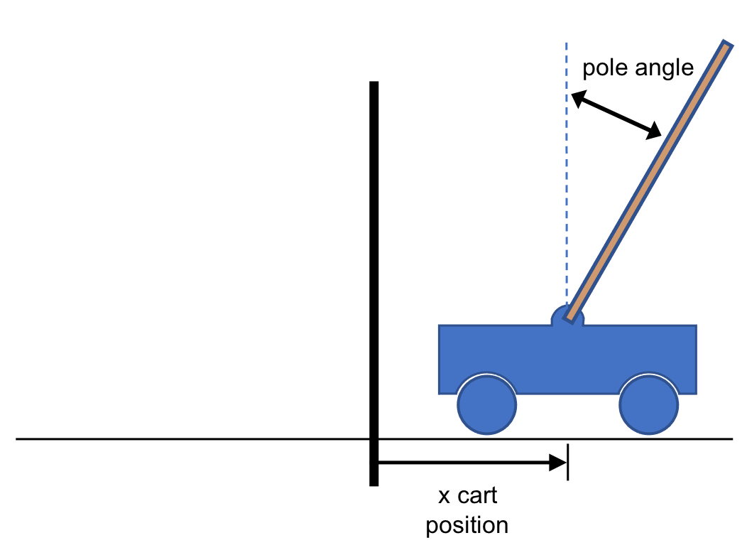
CartPole
The problem we are trying to solve is trying to keep a pole upright. Specifically, the pole is attached by an un-actuated joint to a cart, which moves along a frictionless track. The pendulum starts upright, and the goal is to prevent it from falling over by increasing and reducing the cart's velocity.
Rather than code this environment from scratch, this tutorial will use OpenAI Gym which is a toolkit that provides a wide variety of simulated environments (Atari games, board games, 2D and 3D physical simulations, and so on). Gym makes no assumptions about the structure of your agent (what pushes the cart left or right in this cartpole example), and is compatible with any numerical computation library, such as numpy.
The code below loads the cartpole environment.
import gym
env = gym.make("CartPole-v0")
Let's now start to understand this environment by looking at the action space.
env.action_space
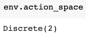
The output Discrete(2) means that there are two actions. In cartpole, 0 corresponds to "push cart to the left" and 1 corresponds to "push cart to the right". Note that in this particular example, standing still is not an option. In reinforcement learning, the agent produces an action output and this action is sent to an environment which then reacts. The environment produces an observation (along with a reward signal, not shown here) which we can see below:
env.reset()
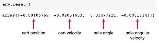
The observation is a vector of dim=4, containing the cart's x position, cart x velocity, the pole angle in radians (1 radian = 57.295 degrees), and the angular velocity of the pole. The numbers shown above are the initial observation after starting a new episode (`env.reset()`). With each timestep (and action), the observation values will change, depending on the state of the cart and pole.
Training an Agent
In reinforcement learning, the goal of the agent is to produce smarter and smarter actions over time. It does so with a policy. In deep reinforcement learning, this policy is represented with a neural network. Let's first interact with the gym environment without a neural network or machine learning algorithm of any kind. Instead we'll start with random movement (left or right). This is just to understand the mechanisms.
The code below resets the environment and takes 20 steps (20 cycles), always taking a random action and printing the results.
# returns an initial observation
env.reset()

for i in range(20):

  # env.action_space.sample() produces either 0 (left) or 1 (right).
  observation, reward, done, info = env.step(env.action_space.sample())

  print("step", i, observation, reward, done, info)

env.close()
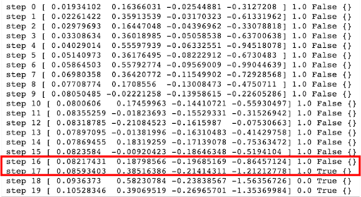
Sample output. There are multiple conditions for episode termination in cartpole. In the image, the episode is terminated because it is over 12 degrees (0.20944 rad). Other conditions for episode termination are cart position is more than 2.4 (center of the cart reaches the edge of the display), episode length is greater than 200, or the solved requirement which is when the average return is greater than or equal to 195.0 over 100 consecutive trials.
The printed output above shows the following things:
- step (how many times it has cycled through the environment). In each timestep, an agent chooses an action, and the environment returns an observation and a reward
- observation of the environment [x cart position, x cart velocity, pole angle (rad), pole angular velocity]
- reward achieved by the previous action. The scale varies between environments, but the goal is always to increase your total reward. The reward is 1 for every step taken for cartpole, including the termination step. After it is 0 (step 18 and 19 in the image).
- done is a boolean. It indicates whether it's time to reset the environment again. Most tasks are divided up into well-defined episodes, and done being True indicates the episode has terminated. In cart pole, it could be that the pole tipped too far (more than 12 degrees/0.20944 radians), position is more than 2.4 meaning the center of the cart reaches the edge of the display, episode length is greater than 200, or the solved requirement which is when the average return is greater than or equal to 195.0 over 100 consecutive trials.
- info which is diagnostic information useful for debugging. It is empty for this cartpole environment.
While these numbers are useful outputs, a video might be clearer. If you are running this code in Google Colab, it is important to note that there is no display driver available for generating videos. However, it is possible to install a virtual display driver to get it to work.
# install dependencies needed for recording videos
!apt-get install -y xvfb x11-utils
!pip install pyvirtualdisplay==0.2.*
The next step is to start an instance of the virtual display.
from pyvirtualdisplay import Display
display = Display(visible=False, size=(1400, 900))
_ = display.start()
OpenAI gym has a VideoRecorder wrapper that can record a video of the running environment in MP4 format. The code below is the same as before except that it is for 200 steps and is recording.
from gym.wrappers.monitoring.video_recorder import VideoRecorder
before_training = "before_training.mp4"

video = VideoRecorder(env, before_training)
# returns an initial observation
env.reset()
for i in range(200):
  env.render()
  video.capture_frame()
  # env.action_space.sample() produces either 0 (left) or 1 (right).
  observation, reward, done, info = env.step(env.action_space.sample())
  # Not printing this time
  #print("step", i, observation, reward, done, info)

video.close()
env.close()

Usually you end the simulation when done is 1 (True). The code above let the environment keep on going after a termination condition was reached. For example, in CartPole, this could be when the pole tips over, pole goes off-screen, or reaches other termination conditions.
The code above saved the video file into the Colab disk. In order to display it in the notebook, you need a helper function.
from base64 import b64encode
def render_mp4(videopath: str) -> str:
  """
  Gets a string containing a b4-encoded version of the MP4 video
  at the specified path.
  """
  mp4 = open(videopath, 'rb').read()
  base64_encoded_mp4 = b64encode(mp4).decode()
  return f'<video width=400 controls><source src="data:video/mp4;' \
         f'base64,{base64_encoded_mp4}" type="video/mp4"></video>'
The code below renders the results. You should get a video similar to the one below.
from IPython.display import HTML
html = render_mp4(before_training)
HTML(html)
Playing the video demonstrates that randomly choosing an action is not a good policy for keeping the CartPole upright.
How to Train an Agent using Ray's RLlib
The previous section of the tutorial had our agent make random actions disregarding the observations and rewards from the environment. The goal of having an agent is to produce smarter and smarter actions over time and random actions don't accomplish that. To make an agent make smarter actions over time, itl needs a better policy. In deep reinforcement learning, the policy is represented with a neural network.
This tutorial will use the RLlib library to train a smarter agent. RLlib has many advantages like:
- Extreme flexibility. It allows you to customize every aspect of the RL cycle. For instance, this section of the tutorial will make a custom neural network policy using PyTorch (RLlib also has native support for TensorFlow).
- Scalability. Reinforcement learning applications can be quite compute intensive and often need to scale-out to a cluster for faster training. RLlib not only has first-class support for GPUs, but it is also built on Ray which makes scaling Python programs from a laptop to a cluster easy.
- A unified API and support for offline, model-based, model-free, multi-agent algorithms, and more (these algorithms won’t be explored in this tutorial).
- Being part of the Ray Project ecosystem. One advantage of this is that RLlib can be run with other libraries in the ecosystem like Ray Tune, a library for experiment execution and hyperparameter tuning at any scale (more on this later).
While some of these features won't be fully utilized in this post, they are highly useful for when you want to do something more complicated and solve real world problems. You can learn about some impressive use-cases of RLlib here.
To get started with RLlib, you need to first install it.
!pip install 'ray[rllib]'==1.6
Now you can train a PyTorch model using the Proximal Policy Optimization (PPO) algorithm. It is a very well rounded, one size fits all type of algorithm which you can learn more about here. The code below uses a neural network consisting of a single hidden layer of 32 neurons and linear activation functions.
import ray
from ray.rllib.agents.ppo import PPOTrainer
config = {
    "env": "CartPole-v0",
    # Change the following line to `“framework”: “tf”` to use tensorflow
    "framework": "torch",
    "model": {
      "fcnet_hiddens": [32],
      "fcnet_activation": "linear",
    },
}
 stop = {"episode_reward_mean": 195}
 ray.shutdown()
ray.init(
  num_cpus=3,
  include_dashboard=False,
  ignore_reinit_error=True,
  log_to_driver=False,
)
# execute training
analysis = ray.tune.run(
  "PPO",
  config=config,
  stop=stop,
  checkpoint_at_end=True,
)
This code should produce quite a bit of output. The final entry should look something like this:
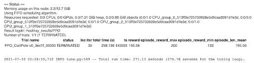
The entry shows it took 35 iterations, running over 258 seconds, to solve the environment. This will be different each time, but will probably be about 7 seconds per iteration (258 / 35 = 7.3). Note that if you like to learn the Ray API and see what commands like ray.shutdown and ray.init do, you can check out this tutorial.
How to use a GPU to Speed Up Training
While the rest of the tutorial utilizes CPUs, it is important to note that you can speed up model training by using a GPU in Google Colab. This can be done by selecting Runtime > Change runtime type and set hardware accelerator to GPU. Then select Runtime > Restart and run all.
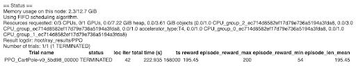
Notice that, although the number of training iterations might be about the same, the time per iteration has come down significantly (from 7 seconds to 5.5 seconds).
Creating a Video of the Trained Model in Action
RLlib provides a Trainer class which holds a policy for environment interaction. Through the trainer interface, a policy can be trained, action computed, and checkpointed. While the analysis object returned from ray.tune.run earlier did not contain any trainer instances, it has all the information needed to reconstruct one from a saved checkpoint because checkpoint_at_end=True was passed as a parameter. The code below shows this.
# restore a trainer from the last checkpoint
trial = analysis.get_best_logdir("episode_reward_mean", "max")
checkpoint = analysis.get_best_checkpoint(
  trial,
  "training_iteration",
  "max",
)
trainer = PPOTrainer(config=config)
trainer.restore(checkpoint)
Let’s now create another video, but this time choose the action recommended by the trained model instead of acting randomly.
after_training = "after_training.mp4"
after_video = VideoRecorder(env, after_training)
observation = env.reset()
done = False
while not done:
  env.render()
  after_video.capture_frame()
  action = trainer.compute_action(observation)
  observation, reward, done, info = env.step(action)
after_video.close()
env.close()
# You should get a video similar to the one below.
html = render_mp4(after_training)
HTML(html)
This time, the pole balances nicely which means the agent has solved the cartpole environment!
Hyperparameter Tuning with Ray Tune
The Ray Ecosystem
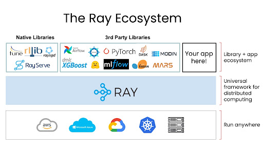
RLlib is a reinforcement learning library that is part of the Ray Ecosystem. Ray is a highly scalable universal framework for parallel and distributed python. It is very general and that generality is important for supporting its library ecosystem. The ecosystem covers everything from training, to production serving, to data processing and more. You can use multiple libraries together and build applications that do all of these things.
This part of the tutorial utilizes Ray Tune which is another library in the Ray Ecosystem. It is a library for experiment execution and hyperparameter tuning at any scale. While this tutorial will only use grid search, note that Ray Tune also gives you access to more efficient hyperparameter tuning algorithms like population based training, BayesOptSearch, and HyperBand/ASHA.
Let’s now try to find hyperparameters that can solve the CartPole environment in the fewest timesteps.
Enter the following code, and be prepared for it to take a while to run:
parameter_search_config = {
    "env": "CartPole-v0",
    "framework": "torch",

    # Hyperparameter tuning
    "model": {
      "fcnet_hiddens": ray.tune.grid_search([[32], [64]]),
      "fcnet_activation": ray.tune.grid_search(["linear", "relu"]),
    },
    "lr": ray.tune.uniform(1e-7, 1e-2)
}

# To explicitly stop or restart Ray, use the shutdown API.
ray.shutdown()

ray.init(
  num_cpus=12,
  include_dashboard=False,
  ignore_reinit_error=True,
  log_to_driver=False,
)

parameter_search_analysis = ray.tune.run(
  "PPO",
  config=parameter_search_config,
  stop=stop,
  num_samples=5,
  metric="timesteps_total",
  mode="min",
)

print(
  "Best hyperparameters found:",
  parameter_search_analysis.best_config,
)
By asking for 12 CPU cores by passing in num_cpus=12 to ray.init, four trials get run in parallel across three cpus each. If this doesn’t work, perhaps Google has changed the VMs available on Colab. Any value of three or more should work. If Colab errors by running out of RAM, you might need to do Runtime > Factory reset runtime, followed by Runtime > Run all. Note that there is an area in the top right of the Colab notebook showing the RAM and disk use.
Specifying num_samples=5 means that you will get five random samples for the learning rate. For each of those, there are two values for the size of the hidden layer, and two values for the activation function. So, there will be 5 * 2 * 2 = 20 trials, shown with their statuses in the output of the cell as the calculation runs.
Note that Ray prints the current best configuration as it goes. This includes all the default values that have been set, which is a good place to find other parameters that could be tweaked.
After running this, the final output might be similar to the following output:
INFO tune.py:549 -- Total run time: 3658.24 seconds (3657.45 seconds for the tuning loop).
Best hyperparameters found: {'env': 'CartPole-v0', 'framework': 'torch', 'model': {'fcnet_hiddens': [64], 'fcnet_activation': 'relu'}, 'lr': 0.006733929096170726};'''
So, of the twenty sets of hyperparameters, the one with 64 neurons, the ReLU activation function, and a learning rate around 6.7e-3 performed best.
Conclusion
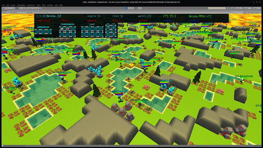
Neural MMO is an environment modeled from Massively Multiplayer Online games — a genre supporting hundreds to thousands of concurrent players. You can learn how Ray and RLlib help enable some key features of this and other projects here.
This tutorial illustrated what reinforcement learning is by introducing reinforcement learning terminology, by showing how agents and environments interact, and by demonstrating these concepts through code and video examples. If you would like to learn more about reinforcement learning, check out the RLlib tutorial by Sven Mika. It is a great way to learn about RLlib’s best practices, multi-agent algorithms, and much more. If you would like to keep up to date with all things RLlib and Ray, consider following @raydistributed on twitter and sign up for the Ray newsletter.
Original. Reposted with permission.
Related:
- Getting Started with Reinforcement Learning
- Facebook Launches One of the Toughest Reinforcement Learning Challenges in History
- 10 Real-Life Applications of Reinforcement Learning