How to Use Permutation Tests
A walkthrough of permutation tests and how they can be applied to time series data.
By Michael Berk, Data Scientist at Tubi
Permutation tests are non-parametric tests that require very few assumptions. So, when you don’t know much about your data generating mechanism (the population), permutation tests are an effective way to determine statistical significance.
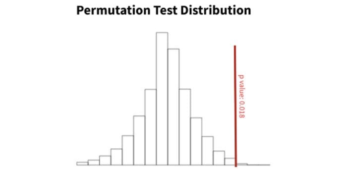
Figure 1: example of a permutation test distribution. The red vertical line is our observed data test statistic. Here, 98.2% of our permutation distribution is below our red line, indicating a p-value of 0.018. Image by author.
A recent paper published by researchers at Stanford extends the permutation testing framework to time series data, an area where permutation tests are often invalid. The method is very mathy and brand new, so there’s little support and no python/R libraries. However, it’s pretty efficient and can be implemented at scale.
In this post we will discuss the basics of permutation tests and briefly outline the time series method.
Let’s dive in.
Technical TLDR
Permutation tests are non-parametric tests that solely rely on the assumption of exchangeability.
To get a p-value, we randomly sample (without replacement) possible permutations of our variable of interest. The p-value is the proportion of samples that have a test statistic larger than that of our observed data.
Time series data is rarely exchangeable. To account for the lack of exchangeability, we divide our test statistic by an estimate of the standard error, thereby converting out test statistic to a t-statistic. This “studentization” process allows us to run autocorrelation tests on non-exchangeable data.
But, how does permutation testing actually work?
Let’s slow down a bit and really understand permutation tests…
Permutation Tests 101
Permutation tests are very simple, but surprisingly powerful.
The purpose of a permutation test is to estimate the population distribution, the distribution where our observations came from. From there, we can determine how rare our observed values are relative to the population.
In figure 2, we see a graphical representation of a permutation test. There are 5 observations, represented by each row, and two columns of interest, Risk and Deaths.
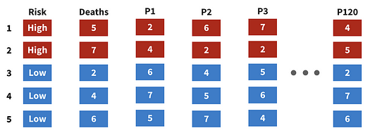
Figure 2: framework for a permutation test. Image by author.
First, we develop many permutations of our variable of interest, labeled P1, P2, …, P120. At the end of this step, we’ll have a large number of theoretical draws from our population. Those draws are then combined to estimate the population distribution.
Note that we will never see a duplicate permutation — permutation tests sample an array of all possible permutations without replacement.
Second, we can calculate our p-value. Using the median as our test statistic (although it can be any statistic derived from our data), we’d follow the steps below:
- Calculate the median of the observed data (the Deaths column).
- For each permutation, calculate the median.
- Determine the proportion of permutation medians that are more extreme than our observed median. That proportion is our p-value.
If you like code, here’s some pythonic pseudocode for calculating the p-value:
permutations = permute(data, P=120)observed_median = median(data)
p_medians = [median(p) for p in permutations]p_val = sum(p > observed_median for p in p_medians) / len(p_medians)
Now that we understand the method, let’s determine when to use it.
Assumptions of a Permutation Test
Permutation tests are appealing because they are non-parametric and only require the assumption of exchangeability. Let’s discuss both concepts in turn.
Parametric methods assume an underlying distribution. Non-parametric methods do not. It’s that simple.
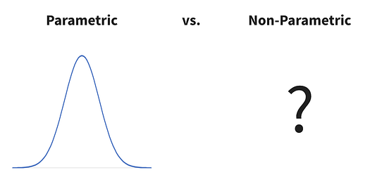
Figure 3: parametric vs non-parametric visualization. Image by author.
Now using parametric methods requires that we’re confident about the distribution of our data. For instance, in A/B tests we can leverage the central limit theorem to conclude that the observed data will exhibit a normal distribution. From there we can run a t-test and get a p-value.
However, in other cases we cannot know the distribution so we must leverage non-parametric methods.
For testing purposes, both parametric and non-parametric methods estimate the population distribution. The main difference is that parametric tests leverage assumptions to create the distribution whereas non-parametric tests leverage resampling.
Great. Let’s move on to exchangeability.
Exchangeability refers to a sequence of random variables. Formally, a sequence is exchangeable if any permutation of that sequence has the same joint probability distribution as the original.
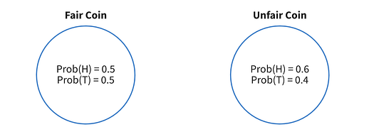
Figure 4: visualization of a fair an biased coin. Image by author.
So, in figure 4 we can see two coins. The left coin is fair with a 50% of getting heads (H) and 50% of getting tails (T). The right coin is biased with a 60% chance of getting heads.
If we were to flip the fair coin many times, we’d have an exchangeable sequence. Likewise, if we flipped the unfair coin many times, we’d have an exchangeable sequence. However, if we alternated between flipping the fair and unfair coin, we would not have an exchangeable sequence.
If the distribution of our data generating mechanism (the coin) changes, our sequence no longer becomes exchangeable.
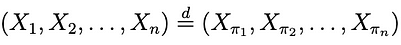
Figure 5: definition of exchangeability. Image by author.
Mathematically, we define exchangeability as shown in figure 5. The sequence on the left is the original data and the sequence on the right is a permutation of the original data. If they have the same distribution, they’re exchangeable.
Permutation Tests for Time Series Dependence
Often, time series data are not exchangeable — prior values can be determinant of future values. If you have strong evidence that your time series data are truly exchangeable, then you can run a regular permutation test, but if not, you’ll need to leverage the below method.
The paper discusses a way to run an autocorrelation test on a time series dataset, but the concepts can generalize to other tests. Also note that autocorrelation is simply the correlation between a value and it’s prior value, for all values.
We going to briefly touch on the method because it’s really really complex. But, the approach is the following:
- Estimate the standard error of our autocorrelation value.
- Convert our statistic to a t-statistic by dividing by the standard error.
- Run a t-test.
Section 2 outlines calculating the standard error, specifically equations 2.9 and 2.12. We are unfortunately not going to cover them here because they’re really long.
Summary and Implementation Notes
There you have it — a walkthrough of permutation tests and some information how they can be applied to non-exchangeable time series data.
To summarize, permutation tests are great because they’re non-parametric and only require the assumption of exchangeability. Permutation tests develop many permutations of our data to estimate the distribution of our population. From there, we can assign a p-value to our observed data. For non-exchangeable time series data, one method is outlined in the paper.
Finally, here are some notes on implementation:
- When there are many rows, you cannot develop all possible permutations. Instead, sample those permutations without replacement to estimate the distribution.
- Permutation tests are effective when there’s a small sample size or when parametric assumptions are not met. Because we only require exchangeability, they’re very robust.
- Permutation tests tend to give larger p-values than parametric tests.
- If your data were randomized in an experiment, you can use a simple randomization test.
- The method for time series autocorrelation requires stationary data. If your data are not stationary, look into differencing.
Thanks for reading! I’ll be writing 34 more posts that bring academic research to the DS industry. Check out my comment for links to the main source for this post and some useful resources.
Bio: Michael Berk (https://michaeldberk.com/) is a Data Scientist at Tubi.
Original. Reposted with permission.
Related:
- How to Find Weaknesses in your Machine Learning Models
- Virtual Presentation Tips for Data Scientists
- 5 Advanced Tips on Python Sequences