Uncertainty Quantification in Artificial Intelligence-based Systems
The article summarizes the plethora of UQ methods using Bayesian techniques, shows issues and gaps in the literature, suggests further directions, and epitomizes AI-based systems within the Financial Crime domain.
Abstract
While Artificial Intelligence (AI) based systems hold great promise and are increasingly employed to assist in a variety of complex tasks, the results are not fully reliable due to the challenges introduced by uncertainty. Uncertainty quantification (UQ) plays a pivotal role in the reduction of uncertainties during both optimization and decision making, applied to solve a variety of real-world applications in science, business, and engineering. This article expediently presents the concepts of uncertainty, its sources, types, and measurements. The article summarizes the plethora of UQ methods using Bayesian techniques, shows issues and gaps in the literature, suggests further directions, and epitomizes AI-based systems within the Financial Crime domain.
Introduction
In recent years, there has been an increased need for the use of AI-based systems which by nature are active systems which required to act automatically based on events or changes in the environment. Such systems span many areas, from active databases to applications that drive the core business processes of today's enterprises. However, in many cases, the events to which the system must respond are not generated by monitoring tools but must be inferred from other events based on complex temporal predicates. Machine Learning (ML) models generate an optimal solution based on their training data. In many applications, such inference is inherently uncertain. However, if the uncertainty in the data and the model parameters are not considered, such optimal solutions have a high risk of failure in actual world deployment.
Typical AI-based system pipelines consist of collecting data, pre-processing it, selecting a model to learn from the data, choosing a learning algorithm to train a selected model, and drawing inferences from the learned model. However, there are inherent uncertainties associated with each of these steps. For example, data uncertainty may arise from the inability to collect or represent real-world data reliably. Flaws in data pre-processing whether, during curation, cleaning, or labeling also create data uncertainty. As models only serve as a proxy for the real world and learning and inference algorithms rely on various simplifying assumptions, they introduce modeling and inferential uncertainties. The predictions made by an AI system are susceptible to all these sources of uncertainty. Reliable uncertainty estimates provide a vital diagnostic for both developers and users of an AI system. For example, high data uncertainty may point towards improving the data representation process, while a high model uncertainty may suggest the need to collect more data. For users, accurate uncertainties, especially when combined with effective communication strategies, can add a critical layer of transparency and trust, crucial for better AI-assisted decision making. Such trust in AI systems is essential for their reliable deployment in high-stakes applications spanning medicine, finance, and the social sciences.
These observations have revitalized my interest in UQ research. Many approaches have been proposed for improved UQ in AI systems, however, choosing a particular UQ method depends on many factors: the underlying model, type of machine learning task (regression vs. classification vs segmentation), characteristics of the data, transparency of the machine learning models and final objectives. If inappropriately used, a particular UQ method may produce poor uncertainty estimates and mislead users. Moreover, even a highly accurate uncertainty estimate may be misleading if poorly communicated.
This article presents an extended introduction to types of uncertainty and characterize its sources, discusses the UQ approaches, formalizes uncertain modeling, and articulates its notion upon complex systems. The article overviews the different approaches used in ML to quantify uncertainty using Bayesian techniques. In addition, there is a focus on the evaluation of uncertainty measurements in different machine learning tasks such as classification, regression, and segmentation. The article provides a term of calibration within UQ methods, enlists open gaps in the literature, demonstrates UQ in a real-world application within the financial crime domain, and formulates a generic evaluation framework for such systems.
Aleatoric Uncertainty
Aleatoric uncertainty (aka statistical uncertainty), and is representative of unknowns that differ each time we run the same experiment. Aleatoric uncertainty refers to the inherent uncertainty due to probabilistic variability. This type of uncertainty is irreducible, in that there will always be variability in the underlying variables. These uncertainties are characterized by a probability distribution. For example, a single arrow shot with a mechanical bow that exactly duplicates each launch (the same acceleration, altitude, direction, and final velocity) will not all impact the same point on the target due to random and complicated vibrations of the arrow shaft, the knowledge of which cannot be determined sufficiently to eliminate the resulting scatter of impact points.
Epistemic Uncertainty
Epistemic uncertainty (aka systematic uncertainty), and is due to things one could in principle know but does not in practice. Epistemic uncertainty is the scientific uncertainty in the model of the process. It is due to limited data and knowledge. The epistemic uncertainty is characterized by alternative models. For discrete random variables, the epistemic uncertainty is modeled by alternative probability distributions. An example of a source of this uncertainty would be the pull in an experiment designed to measure the acceleration of gravity near the earth's surface. The commonly used gravitational acceleration of 9.8 m/s² ignores the effects of air resistance, but the air resistance for the object could be measured and incorporated into the experiment to reduce the resulting uncertainty in the calculation of the gravitational acceleration.
Aleatoric and Epistemic Uncertainty Interaction
Aleatoric and epistemic uncertainty can also occur simultaneously in a single term e.g. when experimental parameters show aleatoric uncertainty, and those experimental parameters are input to a computer simulation. If then for the uncertainty quantification a surrogate model, e.g. a Gaussian process or a Polynomial Chaos Expansion, is learned from computer experiments, this surrogate exhibits epistemic uncertainty that depends on or interacts with the aleatoric uncertainty of the experimental parameters. Such uncertainty cannot solely be classified as aleatoric or epistemic anymore but is a more general inferential uncertainty. In real-life applications, both kinds of uncertainties are present. Uncertainty quantification intends to explicitly express both types of uncertainty separately.
The quantification for the aleatoric uncertainties can be relatively straightforward, where traditional (frequentist) probability is the most basic form. Techniques such as the Monte Carlo method are frequently used. To evaluate epistemic uncertainties, efforts are made to understand the lack of knowledge of the system, process, or mechanism. Epistemic uncertainty is generally understood through the lens of Bayesian probability, where probabilities are interpreted as indicating how certain a rational person could be regarding a specific claim.
Model and Data Uncertainty
The model uncertainty covers the uncertainty that is caused by shortcomings in the model, either by errors in the training procedure, an insufficient model structure, or lack of knowledge due to unknown samples or a bad coverage of the training data set. In contrast to this, data uncertainty is related to uncertainty that directly stems from the data. Data uncertainty is caused by information loss when representing the real world within a data sample and representing the distribution.
For example, in regression tasks noise in the input and target measurements causes data uncertainty that the network cannot learn to correct. In classification tasks, samples that do not contain enough information to identify one class with 100% certainty cause data uncertainty on the prediction. The information loss is a result of the measurement system, e.g. by representing real-world information by image pixels with a specific resolution, or by errors in the labeling process.
While model uncertainty can be (theoretically) reduced by improving the architecture, the learning process, or the training data set, the data uncertainties cannot be explained away.
Predictive Uncertainty
On the basis of the input data domain, the predictive uncertainty can also be classified into three main classes:
- In-domain uncertainty: represents the uncertainty related to an input drawn from a data distribution assumed to be equal to the training data distribution. The in-domain uncertainty stems from the inability of the deep neural network to explain an in-domain sample due to a lack of in-domain knowledge. From a modeler point of view, in domain uncertainty is caused by design errors (model uncertainty) and the complexity of the problem at hand (data uncertainty). Depending on the source of the in-domain uncertainty, it might be reduced by increasing the quality of the training data (set) or the training process.
- Domain-shift uncertainty: denotes the uncertainty related to an input drawn from a shifted version of the training distribution. The distribution shift results from insufficient coverage by the training data and the variability inherent to real-world situations. A domain shift might increase the uncertainty due to the inability of the DNN to explain the domain shift sample-based samples at training time. Some errors causing domain shift uncertainty can be modeled and can therefore be reduced.
- Out-of-domain uncertainty: represents the uncertainty related to an input drawn from the subspace of unknown data. The distribution of unknown data is different and far from the training distribution. For example, when domain-shift uncertainty describes phenomena like a blurred picture of a dog, out-of-domain uncertainty describes the case when a network that learned to classify cats and dogs is asked to predict a bird. The out-of-domain uncertainty stems from the inability of the Deep Neural Networks (DNN) to explain an out-of-domain sample due to its lack of out-of-domain knowledge. From a modeler point of view, out-of-domain uncertainty is caused by input samples, where the network is not meant to give a prediction for or by insufficient training data.
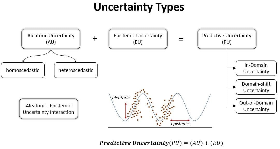 Figure 1: Uncertainty types
Uncertainty versus Variability
Technical professionals are often asked to estimate "ranges" for uncertain quantities. It is important that they distinguish whether they are being asked for variability ranges or uncertainty ranges. Likewise, it is important for modelers to know if they are building models of variability or uncertainty, and their relationship, if any.
Sources of Uncertainty
- Parameter uncertainty: It comes from the model parameters that are input to the mathematical model but whose exact values are unknown to experimentalists and cannot be controlled in physical experiments, or whose values cannot be exactly inferred by statistical methods. For example, local free-fall acceleration in a falling object experiment.
- Parametric variability: it comes from the variability of input variables of the model. For example, the dimensions in a datum may not be exactly as assumed, which would cause variability in the performance of the model trained on this high-dimensional dataset.
- Structural uncertainty: aka model inadequacy, model bias, or model discrepancy, It comes from the lack of knowledge of the underlying physics or principles in the problem. It depends on how accurately a mathematical model describes the true system for a real-life situation, considering the fact that models are almost always only approximations to reality. One example is when modeling the process of a falling object using the free-fall model; the model itself is inaccurate since there always exists air friction. In this case, even if there is no unknown parameter in the model, a discrepancy is still expected between the model and true physics. Structural uncertainty is present when we are uncertain about the model output because we are uncertain about the functional form of the model.
- Algorithmic uncertainty: aka numerical uncertainty, or discrete uncertainty. This type comes from numerical errors and numerical approximations per implementation of the computer model. Most models are too complicated to solve exactly. For example, the finite element method or finite difference method may be used to approximate the solution of a partial differential equation (which introduces numerical errors).
- Experimental uncertainty: aka observation error. It comes from the variability of experimental measurements. The experimental uncertainty is inevitable and can be noticed by repeating a measurement many times using exactly the same settings for all inputs/variables.
- Interpolation uncertainty: This comes from a lack of available data collected from model simulations and/or experimental measurements. For other input settings that don't have simulation data or experimental measurements, one must interpolate or extrapolate in order to predict the corresponding responses.
Types of Problems
There are two major types of problems in uncertainty quantification: one is the forward propagation of uncertainty (where the various sources of uncertainty are propagated through the model to predict the overall uncertainty in the system response) and the other is the inverse assessment of model uncertainty and parameter uncertainty (where the model parameters are calibrated simultaneously using test data).
Forward (propagation of uncertainty)
Uncertainty propagation is the quantification of uncertainties in system output(s) propagated from uncertain inputs. It focuses on the influence on the outputs from the parametric variability listed in the sources of uncertainty. The targets of uncertainty propagation analysis can be:
- Evaluate low-order moments of the outputs, i.e. mean and variance
- Evaluate the reliability of the outputs
- Assess the complete probability distribution of the outputs
Inverse (inverse problem)
Given some experimental measurements of a system and some computer simulation results from its mathematical model, inverse uncertainty quantification estimates the discrepancy between the experiment and the mathematical model (which is called bias correction) and estimates the values of unknown parameters in the model if there are any (which is called parameter calibration or simply calibration).
Generally, this is a much more difficult problem than forwarding uncertainty propagation; however, it is of great importance since it is typically implemented in a model updating process. There are several scenarios in inverse uncertainty quantification:
- Bias correction only: bias correction quantifies the model inadequacy, i.e. the discrepancy between the experiment and the mathematical model
- Parameter calibration only: parameter calibration estimates the values of one or more unknown parameters in a mathematical model.
- Bias correction and parameter calibration: considers an inaccurate model with one or more unknown parameters, and its model updating formulation combines the two together: It is the most comprehensive model updating formulation that includes all possible sources of uncertainty, and it requires the most effort to solve.
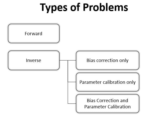 Figure 2: Types of Problems within uncertainty quantification
Mathematical Formalization
As we say previously (Figure 1), predictive uncertainty consists of two parts: epistemic uncertainty, and aleatoric uncertainty, which can be written as a sum of these two parts:

Epistemic uncertainties can be formulated as a probability distribution over model parameters.
Let

denotes a training dataset with inputs

where C represents the number of classes. The aim is to optimize the parameters


For classification, the softmax likelihood can be used:

Eq.1
and the Gaussian likelihood can be assumed for regression:

Eq.2

By applying Bayes’ theorem can be written as follows:

Eq.3


Eq.4
This process is called inference or marginalization. However,

cannot be computed analytically, but it can be approximated by variational parameters

The aim is to approximate a distribution that is close to the posterior distribution obtained by the model. As such, the Kullback-Leibler (KL) divergence is needed to be minimized with regard to ?. The level of similarity among the two distributions can be measured as follows:

Eq.5
The predictive distribution can be approximated by minimizing KL divergence, as follows:

Eq.6
where

indicates the optimized objective. KL divergence minimization can also be rearranged into the evidence lower bound (ELBO) maximization:

Eq.7
where

is able to describe the data well by maximizing the first term, and being as close as possible to the prior by minimizing the second term. This process is called variational inference (VI). Dropout VI is one of the most common approaches that has been widely used to approximate inference in complex models. The minimization objective is as follows:

Eq.8
where N and P represent the number of samples and dropout probability, respectively. To obtain data-dependent uncertainty, the precision ? in (Eq.2) can be formulated as a function of data. One approach to obtain epistemic uncertainty is to mix two functions:


A prior distribution is placed over the weights of the model, and then the amount of change in the weights for given data samples is computed. The Euclidian distance loss function can be adapted as follows:

Eq.9
The predictive variance can be obtained as follows:

Eq.10
Selective Methodologies
Much research has been done to solve uncertainty quantification problems, though a majority of them deal with uncertainty propagation. During the past one to two decades, a number of approaches for inverse uncertainty quantification problems have also been developed and have proved to be useful for most small- to medium-scale problems.
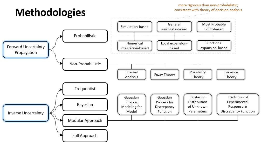
Figure 3: Selective methodologies for uncertainty quantification
Forward Propagation
- Simulation-based methods: Monte Carlo simulations, importance sampling, adaptive sampling, etc.
- General surrogate-based methods: In a non-intrusive approach, a surrogate model is learned in order to replace the experiment or the simulation with a cheap and fast approximation. Surrogate-based methods can also be employed in a fully Bayesian fashion. This approach has proven particularly powerful when the cost of sampling, e.g. computationally expensive simulations, is prohibitively high.
- Local expansion-based methods: Taylor series, perturbation method, etc. These methods have advantages when dealing with relatively small input variability and outputs that don't express high nonlinearity. These linear or linearized methods are detailed in the article Uncertainty propagation.
- Functional expansion-based methods: Neumann expansion, orthogonal or Karhunen–Loeve expansions (KLE), with polynomial chaos expansion (PCE) and wavelet expansions as special cases.
- Most probable point (MPP)-based methods: first-order reliability method (FORM) and second-order reliability method (SORM).
- Numerical integration-based methods: Full factorial numerical integration (FFNI) and dimension reduction (DR).
For non-probabilistic approaches, interval analysis, Fuzzy theory, possibility theory, and evidence theory are among the most widely used.
The probabilistic approach is considered the most rigorous approach to uncertainty analysis in engineering design due to its consistency with the theory of decision analysis. Its cornerstone is the calculation of probability density functions for sampling statistics. This can be performed rigorously for random variables that are obtainable as transformations of Gaussian variables, leading to exact confidence intervals.
Inverse Uncertainty
- Frequentist: standard error of parameter estimates is readily available, which can be expanded into a confidence interval.
- Bayesian: Several methodologies for inverse uncertainty quantification exist under the Bayesian framework. The most complicated direction is to aim at solving problems with both bias correction and parameter calibration. The challenges of such problems include not only the influences from model inadequacy and parameter uncertainty but also the lack of data from both computer simulations and experiments. A common situation is that the input settings are not the same over experiments and simulations. Another common situation is that parameters derived from experiments are input to simulations. For computationally expensive simulations, then often a surrogate model, e.g. a Gaussian process or a Polynomial Chaos Expansion, is necessary, defining an inverse problem for finding the surrogate model that best approximates the simulations.
- Modular approach: An approach to inverse uncertainty quantification is the modular Bayesian approach. The modular Bayesian approach derives its name from its four-module procedure. Apart from the currently available data, the prior distribution of unknown parameters should be assigned.
- Gaussian process modeling for the model: To address the issue from lack of simulation results, the computer
model is replaced with a Gaussian process (GP) model - Gaussian process modeling for discrepancy function: Similarly, with the first module, the discrepancy
function is replaced with a GP model - Posterior distribution of unknown parameters: Bayes' theorem is applied to calculate the posterior
distribution of the unknown parameters: - Prediction of the experimental response and discrepancy function
- Gaussian process modeling for the model: To address the issue from lack of simulation results, the computer
- Full approach: Fully Bayesian approach requires that not only the priors for unknown parameters but also the priors for the other hyperparameters should be assigned.
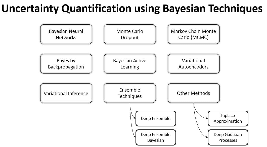
Figure 4: Uncertainty quantification using Bayesian Techniques
Uncertainty Quantification in Machine Learning
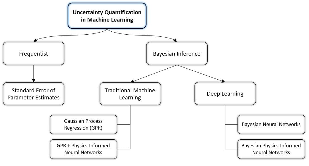
Figure 5: Taxonomy of Uncertainty Quantification in Machine Learning
Evaluating Classification
- Measuring Data Uncertainty in Classification Tasks: given prediction, probability vector represents a categorical distribution, i.e. it assigns a probability to each class to be the correct prediction. Since the prediction is not given as an explicit class but as a probability distribution, uncertainty estimates can be directly derived from the prediction. In general, this pointwise prediction can be seen as estimated data uncertainty. However, the model’s estimation of the data uncertainty is affected by model uncertainty, which has to be taken into account separately. In order to evaluate the amount of predicted data uncertainty, one can for example apply the maximal class probability or the entropy measures. The maximal probability represents a direct representation of certainty, while entropy describes the average level of information in a random variable. Though, one cannot tell from a single prediction how large the amount of model uncertainty is that affects this specific prediction as well.
- Measuring Model Uncertainty in Classification Tasks: an approximated posterior distribution on the learned model parameters can help to receive better uncertainty estimates. With such a posterior distribution, it is possible to evaluate variation i.e. uncertainty of a random variable. The most common measures for this are the mutual information (MI), Expected Kullback-Leibler Divergence (EKL), and the predictive variance. Basically, all these measures compute the expected divergence between the stochastic output and the expected output. MI is minimal when the knowledge about model parameters does not increase the information in the final prediction. Therefore, the MI can be interpreted as a measure of model uncertainty. The Kullback-Leibler divergence measures the divergence between two given probability distributions. The EKL can be used to measure the (expected) divergence among the possible outputs, which can also be interpreted as a measure of uncertainty on the model’s output and therefore represents the model uncertainty. And even for an analytically described distribution, the propagation of the parameter uncertainty into the prediction is in almost all cases intractable and has to be approximated for example with Monte Carlo approximation.
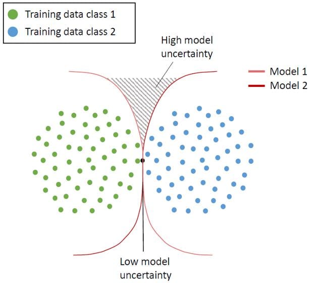
Figure 6: Visualization of the model and the distributional uncertainty for classification models. Source: A Survey of Uncertainty in Deep Neural Networks, Jakob Gawlikowski et. al 2022
- Measuring Distributional Uncertainty in Classification Tasks: Although these uncertainty measures are widely used to capture the variability among several predictions derived from Bayesian neural networks, ensemble methods cannot capture distributional shifts in the input data or out-of-distribution examples, which could lead to a biased inference process and a falsely stated confidence. If all predictors attribute a high probability mass to the same (false) class label, this induces a low variability among the estimates. Hence, the system seems to be certain about its prediction, while the uncertainty in the prediction itself is also evaluated below.
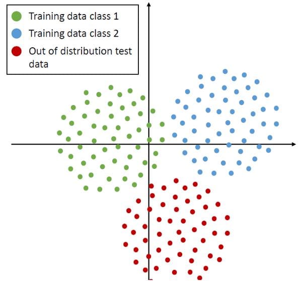
Figure 7: Visualization of the model and the distributional uncertainty for classification models. Source: A Survey of Uncertainty in Deep Neural Networks, Jakob Gawlikowski et. al 2022
- Performance Measure on Complete Data Set: while the measures described above evaluate the performance of individual predictions, others evaluate the usage of these measures on a set of samples. Measures of uncertainty can be used to separate between correctly and falsely classified samples or between in-domain and out-of-distribution samples. For that, the samples are split into two sets, for example in-domain and out-of-distribution or correctly classified and falsely classified. The two most common approaches are the Receiver Operating Characteristic (ROC) curve and the Precision-Recall (PR) curve. Both methods generate curves based on different thresholds of the underlying measure. While the ROC and PR curves give a visual idea of how well the underlying measures are suited to separate the two considered test cases, they do not give a qualitative measure. To reach this, the area under the curve (AUC) can be evaluated. Roughly speaking, the AUC gives a probability value that a randomly chosen positive sample leads to a higher measure than a randomly chosen negative example.
Evaluating Regression
- Measuring Data Uncertainty in Regression Predictions: in contrast to classification tasks, regression tasks only predict a pointwise estimation without any hint of data uncertainty. A common approach to overcome this is to let the network predict the parameters of a probability distribution, for example, a mean vector and a standard deviation for a normally distributed uncertainty. Doing so, a measure of data uncertainty is directly given. The prediction of the standard deviation allows an analytical description that the (unknown) true value is within a specific region. The interval that covers the true value with a certain probability (under the assumption that the predicted distribution is correct) is the quantile function, the inverse of the cumulative probability function. For a given probability value the quantile function gives a boundary. Quantiles assume some probability distribution and interpret the given prediction as to the expected value of the distribution.
In contrast to this, other approaches directly predict a so-called prediction interval (PI) in which the prediction is assumed to lay. Such intervals induce uncertainty as a uniform distribution without giving a concrete prediction. The certainty of such approaches can, as the name indicates, be directly measured by the size of the predicted interval. The Mean Prediction Interval Width (MPIW) can be used to evaluate the average certainty of the model. In order to evaluate the correctness of the predicted intervals the Prediction Interval Coverage Probability (PICP) can be applied. The PCIP represents the percentage of test predictions that fall into a prediction interval
- Measuring Model Uncertainty in Regression Predictions: model uncertainty is mainly caused by the model’s architecture, the training process, and underrepresented areas in the training data. Hence, there is no real difference in the causes and effects of model uncertainty between regression and classification tasks such that model uncertainty in regression tasks can be measured equivalently as already described for classification tasks, i.e. in most cases by approximating an average prediction and measuring the divergence among the single predictions.
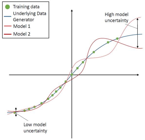
Figure 8: Visualization of the model and the distributional uncertainty for regression models. Source: A Survey of Uncertainty in Deep Neural Networks, Jakob Gawlikowski et. al 2022
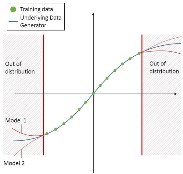
Figure 9: Visualization of the model and the distributional uncertainty for regression models. Source: A Survey of Uncertainty in Deep Neural Networks, Jakob Gawlikowski et. al 2022
- Evaluating Uncertainty in Segmentation Tasks: evaluation of uncertainties in segmentation tasks is very similar to the evaluation for classification problems. The uncertainty is estimated in segmentation tasks using approximates of Bayesian inference. In the context of segmentation, the uncertainty in pixel-wise segmentation is measured using confidence intervals, the predictive variance, the predictive entropy, or the mutual information (MI). The uncertainty in structure estimation is obtained by averaging over all pixel-wise uncertainty estimates. The quality of volume uncertainties is assessed by evaluating the coefficient of variation, the average Dice score, or the intersection over the union. These metrics measure the agreement in area overlap between multiple estimates in a pairwise fashion. Ideally, a false segmentation should result in an increase in pixel-wise and structure uncertainty. To verify whether this is the case, the true positive rate at pixel level should be evaluated and the false detection rate as well as the ROC curves for the retained pixels at different uncertainty thresholds.
Calibration
A predictor is called well-calibrated if the derived predictive confidence represents a good approximation of the actual probability of correctness. Therefore, in order to make use of uncertainty quantification methods, one has to be sure that the system is well calibrated. For regression tasks, the calibration can be defined such that predicted confidence intervals should match the confidence intervals empirically computed from the dataset.
In general, calibration errors are caused by factors related to model uncertainty. This is intuitively clear, since as data uncertainty represents the underlying uncertainty that an input x and a target y represent the same real world information. Following, correctly predicted data uncertainty would lead to a perfectly calibrated system. This is clear, since these methods quantify model and data uncertainty separately and aim at reducing the model uncertainty on the predictions. Besides the methods that improve the calibration by reducing the model uncertainty, a large and growing body of literature has investigated methods for explicitly reducing calibration errors. These methods are presented in the following, followed by measures to quantify the calibration error. It is important to note that these methods do not reduce the model uncertainty, but propagate the model uncertainty onto the representation of the data uncertainty.
For example, if a binary classifier is overfitted and predicts all samples of a test set as class A with probability 1, while half of the test samples are actually class B, the recalibration methods might map the network output to 0.5 in order to have reliable confidence. This probability of 0.5 is not equivalent to the data uncertainty but represents the model uncertainty propagated onto the predicted data uncertainty.
Calibration Methods
Calibration methods can be classified into three main groups according to the step when they are applied:
- Regularization methods applied during the training phase: these methods modify the objective, optimization, and/or regularization procedure in order to build systems and networks that are inherently calibrated.
- Post-processing methods applied after the training process of the model: these methods require a held-out calibration data set to adjust the prediction scores for recalibration. They only work under the assumption that the distribution of the left-out validation set is equivalent to the distribution, on which inference is done. Hence, also the size of the validation data set can influence the calibration result.
- Neural network uncertainty estimation methods: Approaches, that reduce the amount of model uncertainty on a neural network’s confidence prediction, also lead to a better-calibrated predictor. This is because the remaining predicted data uncertainty better represents the actual uncertainty on the prediction. Such methods are based for example on Bayesian methods or deep ensembles (Figure 4).
Real-World Applications
Using innovative technology to protect institutions and safeguard both consumers' and investors' assets, NICE Actimize identifies financial crime, preventing fraud and providing regulatory compliance. It provides real-time, cross-channel fraud prevention, anti-money laundering detection, and trading surveillance solutions that address payment fraud, cybercrime, sanctions monitoring, market abuse, customer due diligence, and insider trading. AI-based systems and advanced analytics solutions find abnormal behavior earlier and faster, eliminating financial losses from theft to fraud, regulatory penalties to sanctions. As a result, organizations reduce losses, increase investigator efficiency, and improve regulatory compliance and oversight.
With the increasing usage of AI-based systems within financial crime, quantifying and handling uncertainties has become more and more important. On one hand, uncertainty quantification plays an important role in risk minimization, which is needed in fraud prevention. On the other hand, there are challenging data sources that provide augmentation for fraud investigations, which are hard to verify. This makes the generation of trustworthy ground truth a very challenging task.
Actimize’s Generic Evaluation Framework
To cope with such issues, Actimize provides an evaluation protocol containing various concrete baseline datasets and evaluation metrics that cover all types of uncertainty that help to boost research in uncertainty quantification. Also, the evaluation with regard to risk-averse and worst-case scenarios is considered as well. Such a general protocol enables data scientist researchers to easily compare different types of methods against an established benchmark as well as on real world datasets.
Conclusion
Uncertainty quantification is one of the key parts of AI-based systems and decision-making processes. The UQ methods are becoming popular to evaluate uncertainty in various real-life applications. Nowadays, uncertainty has become an inseparable part of traditional machine and deep leering methods. This article has comprehensively reviewed the most important UQ concepts and methods that have been applied in traditional machine learning and deep learning.
References
- A. Ashukha, A. Lyzhov, D. Molchanov, and D. Vetrov, “Pitfalls of in-domain uncertainty estimation and Ensembling in deep learning,” in International Conference on Learning Representations, 2020.
- A. G.Wilson and P. Izmailov, “Bayesian deep learning and a probabilistic perspective of generalization,” in Advances in Neural Information Processing Systems, H. Larochelle, M. Ranzato, R. Hadsell, M. F. Balcan, and H. Lin, Eds., vol. 33, 2020, pp. 4697–4708.
- A. Kendall and Y. Gal, “What uncertainties do we need in bayesian deep learning for computer vision?” in Advances in neural information processing systems, 2017, pp. 5574–5584.
- A. Kristiadi, M. Hein, and P. Hennig, “Learnable uncertainty under Laplace approximations,” arXiv preprint arXiv:2010.02720, 2020.
- A. Loquercio, M. Segu, and D. Scaramuzza, “A general framework for uncertainty estimation in deep learning,” IEEE Robotics and Automation Letters, vol. 5, no. 2, pp. 3153–3160, 2020
- A. Malinin and M. Gales, “Predictive uncertainty estimation via prior networks,” in Advances in Neural Information Processing Systems, 2018, pp. 7047–7058.
- Chen, Wang, and Cho 2017 Chen, F.; Wang, C.; and Cho, J.-H. 2017. Collective subjective logic: Scalable uncertainty-based opinion inference. In 2017 IEEE International Conference on Big Data (Big Data), 7–16.
- G. Kahn, A. Villaflor, V. Pong, P. Abbeel, and S. Levine, “Uncertainty-aware reinforcement learning for collision avoidance,” arXiv preprint arXiv:1702.01182, 2017.
- G. Wang, W. Li, M. Aertsen, J. Deprest, S. Ourselin, and T. Vercauteren, “Aleatoric uncertainty estimation with test-time augmentation for medical image segmentation with convolutional neural networks,” Neurocomputing, vol. 338, pp. 34–45, 2019.
- J. Van Amersfoort, L. Smith, Y. W. Teh, and Y. Gal, “Uncertainty estimation using a single deep deterministic neural network,” in Proceedings of the 37th International Conference on Machine Learning. PMLR, 2020, pp. 9690–9700.
- J. Zeng, A. Lesnikowski, and J. M. Alvarez, “The relevance of bayesian layer positioning to model uncertainty in deep bayesian active learning,” arXiv preprint arXiv:1811.12535, 2018.
- Jha, A.; Chandrasekaran, A.; Kim, C.; Ramprasad, R. Impact of dataset uncertainties on machine learning model predictions: The example of polymer glass transition temperatures. Model. Simul. Mater. Sci. Eng. 2019, 27, 024002.
- Jøsang 2016 Jøsang, A. 2016. Subjective Logic: A Formalism for Reasoning Under Uncertainty. Springer.
- Lele, S.R. How Should We Quantify Uncertainty in Statistical Inference? Front. Ecol. Evol. 2020, 8.
- M. S. Ayhan and P. Berens, “Test-time data augmentation for estimation of heteroscedastic aleatoric uncertainty in deep neural networks,” in Medical Imaging with Deep Learning Conference, 2018.
- Meyer, V.R. Measurement uncertainty. J. Chromatogr. A 2007, 1158, 15–24.
- Senel, O. Infill Location Determination and Assessment of Corresponding Uncertainty. Ph.D. Thesis, Texas A & M University, College Station, TX, USA, 2009.
- Siddique, T.; Mahmud, M.S. Classification of fNIRS Data Under Uncertainty: A Bayesian Neural Network Approach 2021. Available online: https://ieeexplore.ieee.org/document/9398971 (accessed on 20 November 2021)
- T. Tsiligkaridis, “Failure prediction by confidence estimation of uncertainty-aware Dirichlet networks,” in 2021 IEEE International Conference on Acoustics, Speech and Signal Processing. IEEE, 2021, pp. 3525–3529.
- Y. Feldman and V. Indelman, “Bayesian viewpoint-dependent robust classification under model and localization uncertainty,” in 2018 IEEE International Conference on Robotics and Automation. IEEE, 2018, pp. 3221–3228.
- Y. Gal and Z. Ghahramani, “Dropout as a bayesian approximation: Representing model uncertainty in deep learning,” in international conference on machine learning, 2016, pp. 1050–1059.
Danny Butvinik is the Chief Data Scientist at NICE Actimize, providing technical and professional leadership. Butvinik is an expert in Artificial Intelligence and Data Science with demonstrated ability in building a data science vision and communicating data-driven analytics to all company departments. Butvinik has a strong focus on anomaly detection in data streams and online machine learning. He regularly publishes academic papers and research articles.
