SQL Window Functions
In this article, we’ll go over SQL window functions and how to use them when writing SQL queries.

Introduction
Writing well-structured, efficient SQL queries is no easy task. It requires a thorough knowledge of all SQL functions and statements, so that you can apply them in your everyday job to solve problems efficiently. In this article, we’ll talk about SQL window functions, which offer a lot of utility to solve common problems, but they are often overlooked.
SQL window functions are very versatile, and can be used to address many different problems in SQL.
Almost all companies ask interview questions that require at least some knowledge of window functions to answer. So if you’re preparing for a data science interview, it’s a good idea to refresh your knowledge of window functions in SQL. In this article, we will focus on the basics. If you’d like to gain a deeper understanding, read this ultimate guide to SQL window functions.
Having a good grasp of window functions can also help you write efficient and optimized SQL queries to address problems you encounter in your everyday job.
What is a Window Function in SQL?
In simple words, window functions in SQL are used to access all other rows of the table to generate a value for the current row.
SQL Window functions get their name because their syntax allows you to define a specific portion, or window of data to work on. First, we define a function, which will run on all rows, and then we use the OVER clause to specify the window of data.

Window functions are considered an ‘advanced’ feature of SQL. At first glance, junior data scientists might be scared by the syntax, but with a little practice, SQL window functions can become much less scary.
SQL Window Function Types
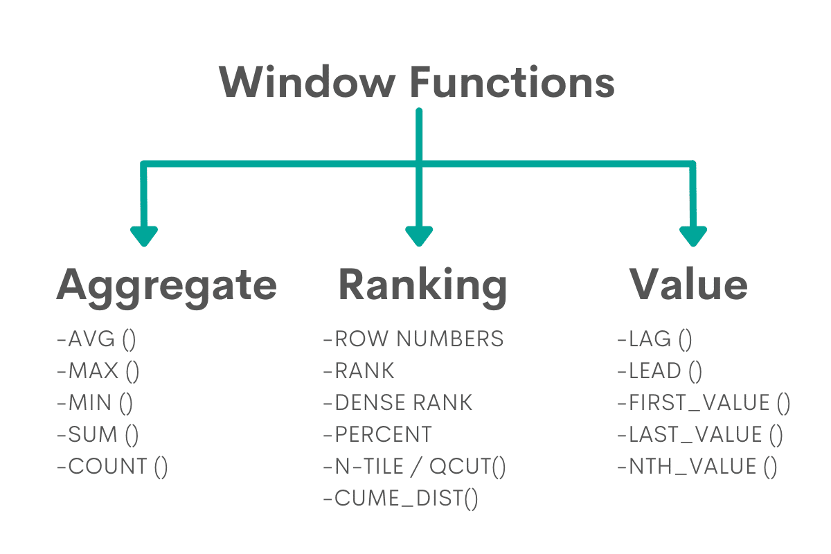
Aggregate Window Functions are necessary to do calculations or find the lowest or highest extremes of data within the window of data. These are the same as regular aggregate functions, but they are applied to specific windows of data, so their behavior is different.
Ranking Window Functions give us the ability to assign rank numbers to a window of data. Each of the 6 major functions ranks rows differently. The ranking also depends on the use of ORDER BY statement.
Value Window Functions allow us to find the values based on their position relative to the current row. They are useful for getting the value from previous or following rows, and for analysis of time-series data.
This is just a short overview of three types of SQL window functions. We’ll discuss them in detail in later parts of the article.
How and When To Use Them?
Once you understand all the window functions and their use cases, it will become a powerful tool at your disposal. They can save you from writing many unnecessary lines of code to solve the problems that can be solved by a single window function.
SQL Window Functions VS Group By Statement
Beginners who read the description of window functions are often confused about what it’s supposed to do and how they’re different from the Group By statement, which seems to work in the exact same way. However, the confusion will go away if you write window functions and see their actual output.
The most significant difference between the Window functions and the Group By statement is that the former allows us to summarize the values while keeping all of the original data. The GROUP BY statement also lets us generate the aggregate values, but the rows are collapsed into a few groups of data.
Use Cases
Getting a job as a data scientist is only the beginning. In your everyday job you’ll encounter problems that need to be solved efficiently. Window functions are very versatile and they will be invaluable as long as you know how to use them.
For instance, if you’re working for a company like Apple, you might need to analyze inner sales data to find the most popular, or the least popular products in their portfolio. One of the most common use cases of window functions is to track time-series data. For instance, you might have to calculate month-over-month growth or decline of specific Apple products, or bookings on Airbnb platform.
Data scientists who work for SaaS companies are often tasked with calculating user churn rate, and track its changes over time. As long as you have user data, you can use window functions to keep track of churn rate.
Aggregate window functions, such as SUM() can be useful for calculating running totals. Let’s imagine that we have sales data for all 12 months of the year. With window functions, we can write a query to calculate a running total (current month + the total of previous months) of the sales data.
Window functions have many other use cases. For example, if you’re working with user data, you can order users by when they signed up, the number of sent messages or other similar metrics.
Window functions also allow us to keep track of health statistics, such as changes in the virus spread, the severity of cases, or other similar insights.
With Other SQL Keywords
In order to effectively use window functions, you must first understand the order of operations in SQL. You can only use window functions with the operations that come after the window functions, not before them. In accordance with this rule, it’s possible to use window functions with the SELECT and ORDER BY statements, but not with others, such as WHERE and GROUP BY.
Typically SQL developers use window functions with the SELECT statement, and the main query can include the ORDER BY statement.
Ranking Window Functions in SQL
These functions allow SQL developers to assign numerical rank to rows.
There are six functions of this type:
ROW_NUMBER() simply numerates the rows starting from 1. The order of rows depends on the ORDER BY statement. If there is none, the ROW_NUMBER() function will simply numerate the rows in their initial state.
RANK() is a more nuanced version of the ROW_NUMBER() function. RANK() considers if the values are equal and assigns them the same rank. For instance, if the values in the third and fourth rows are equal, it will assign them both ranks of three, and, starting from the fifth row, it will continue counting from 5.
DENSE_RANK() works just like the RANK() function, except for one difference. In the same example, if the values in third and fourth columns are tied, both will be assigned the rank of three. However, the fifth row will not start counting from 5, but from 4, considering the fact that previous rows have a rank of three. To learn more about the differences, check this post ? An Introduction to the SQL Rank Functions.
PERCENT_RANK() uses a different approach to ranking. It creates a new column to display the rank values in percentages (from 0 to 1).
NTILE() is a function that takes one numerical argument, which will create batches to divide the data. For instance, NTILE(20) will create 20 buckets of rows, and assign the rank accordingly.
CUME_DIST() function calculates cumulative distribution of the current row. In other words, it goes through every record in the window and returns the portion of the rows with values that are less than or equal to the value in the current row. The relative size of these rows is between 0 (none) and 1 (all).
Ranking Data With RANK()
Ranking Window Functions often come up during the interviews at major tech companies. For example, interviewers at Facebook/Meta often ask candidates to find the most active users on Messenger.
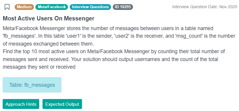
To answer this question, we must first look at the available data. We have one table with multiple different columns. The values of user1 and user2 columns are usernames, and the msg_count column represents the number of messages exchanged between them. According to the name of the question, we must find the users with the highest number of recorded activities. To do that, we must first think about what the activity is: in this context, both sending and receiving a message counts as an activity.
After looking at the data, we see that the msg_count does not represent a total number of messages sent and received by each user in the record. There may be other users they are chatting with. In order to get the total number of activities for each user, we must get the value in the msg_count column where they are at least on the sending or receiving end of the messages.
Let’s take a look at the sample of data from this task:
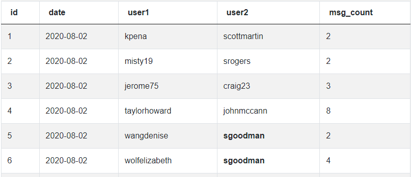
As you can see, the user called sgoodman is a part of two conversations - one is with the username wangdenise and the other with wolfelizabeth. In real life, people can have online conversations with dozens of people. Our query should capture the number of messages exchanged between them.
Solution
Step 1: Combine users in one column
First, we select usernames in the user1 column with their corresponding msg_count value. Then we do the same for users in the user2 column and combine them in one column. We use the UNION ALL operator to do so. This will ensure that all of the users, with their corresponding, sent or received msg_count values are kept in place.
SELECT user1 AS username,
       msg_count
FROM fb_messages
UNION ALL
SELECT user2 AS username,
       msg_count
FROM fb_messages
We must keep in mind that in order for UNION ALL statements to combine the values, the number of columns in both SELECT statements and their respective value types must be the same. So we use the AS statement to rename them to username.
If we run this code, we’ll get the following result:

Step 2: Order the users in decreasing order
Once we have the list of all the users, we must select the username column from the above table and add up the msg_count values of every individual user.
Then we’ll use the RANK() window function to enumerate every record. In this case, we want to use this specific function, instead of DENSE_RANK() because of possible ties in the number of messages within the TOP 10.
The accuracy of ranking window functions depends on the ORDER BY statement, which is used to arrange the values within the window of input data, not the output of the function. In this case, we must use the DESC keyword to make sure that the number of messages is arranged in descending order. This way, RANK() function is applied to the highest input values first.
The OVER keyword is an essential part of window functions syntax. It is used to connect the ranking function to the window of data.
So far, our SQL query should look something like this:
WITH sq AS
  (SELECT username,
          sum(msg_count) AS total_msg_count,
          rank() OVER (
                       ORDER BY sum(msg_count) DESC)
   FROM
     (SELECT user1 AS username,
             msg_count
      FROM fb_messages
      UNION ALL SELECT user2 AS username,
                       msg_count
      FROM fb_messages) a
   GROUP BY username)
To solve our question, we must find the 10 most active users. Using the RANK() window function is necessary to handle the cases when there are any ties within that group of 10 users.
Step 3: Display the TOP 10
In the final step, we should get username and total_msg_count values from the sq subquery, and display the ones that have a rank value of 10 or less. Then arrange them in descending order.
(SELECT username,
          sum(msg_count) AS total_msg_count,
          rank() OVER (
                       ORDER BY sum(msg_count) DESC)
   FROM
     (SELECT user1 AS username,
             msg_count
      FROM fb_messages
      UNION ALL SELECT user2 AS username,
                       msg_count
      FROM fb_messages) a
   GROUP BY username)
SELECT username,
       total_msg_count
FROM sq
WHERE rank <= 10
ORDER BY total_msg_count DESC
If we run this code, we’ll see that it works as it should. And we potentially avoid any errors in case some of the users had identical total_msg_count values.

Finding the Top 5 Percentile Values
Here is an example of another interview question asked at Netflix. A fictional insurance company has developed an algorithm to determine the chances of an insurance claim being fraudulent. Candidates must find the claims in the TOP 5 percentile that are the most likely to be a fraud.

As you might’ve noticed, this question revolves around finding percentile values. The easiest way to do so is using the NTILE() ranking window function in SQL. In this case, we are looking for a percentile value, so the argument to NTILE() would be 100.
The instructions say that we have to identify the top 5 percentile of fraudulent claims from each state. To do that, our window definition should include the PARTITION BY statement. Partition is a way to specify how to group values within the window. For instance, if you had a spreadsheet of users, you could partition them based on the month they signed up.
In this case, we must partition the values in the state column. This means calculating percentiles of each claim from each state. We use the ORDER BY statement to arrange the values in the fraud_score column in descending order.
Note that because the ORDER BY and PARTITION BY statements are used within the window definition, they only apply to each ‘group’ of records, each group representing one state. For instance, the records from California are arranged based on the value in their fraud_score column, the rows with highest values coming first. As soon as there are no more rows for California, the order is reset and starts over from the highest scoring record in another state, Florida.

Finding the Nth Highest Value
There is another question, often asked at Amazon to gauge the candidate’s proficiency in Ranking Window Functions. The task is simple: you are given a single table with many different columns. The question asks us to find the second highest salary of all employee records. After analyzing the available data, it becomes obvious that the most important is the salary column.
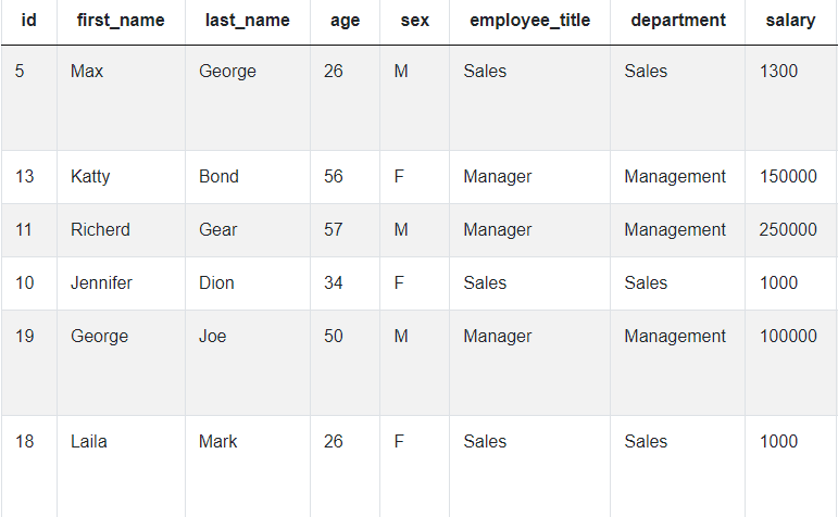
In this case, the wording of the question tells us to find the second highest salary at the company. So if five employees all have a salary of 100 000$ per year, and it is the highest salary, we’ll have to access the sixth employee, who is next in the descending order of salaries.
If you look at the current solution on StrataScratch, we use the DENSE_RANK() window function to get the second-highest value. Also, we use the DISTINCT keyword to weed out duplicates, in case multiple employees have the same salary. We want to rank every remaining record individually, so there’s no need to use the PARTITION BY statement to separate groups of employees.
Aggregate Window Functions in SQL
The default behavior of aggregate functions in SQL is to aggregate the data of all records into a few groups. However, when used as window functions, all rows are kept intact. Instead, aggregate window functions create a separate column for storing the results of aggregation.
There are five aggregate window functions:
AVG() - returns the average of values in a specific column or subset of data
MAX() - returns the highest value in a specific column or subset of data
MIN() - returns the lowest value in a specific column or subset of data
SUM() - returns the sum of all values in a specific column or subset of data
COUNT() - returns the number of rows in a column or a subset of data
Interview questions often revolve around aggregate window functions. For instance, it’s a common task to calculate a running sum and create a new column to display the running sum for every record. For common uses of this SQL window function during interviews, refer to this ultimate guide to SQL aggregate functions.
Finding the Latest Date
To better understand aggregate window functions, let’s look at one interview question from Credit Karma.
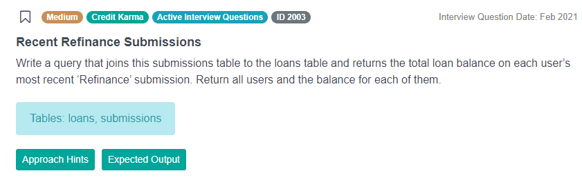
In this question, we have to find and output the most recent balance for every user’s ‘Refinance’ submission. To better understand the question, we must analyze the available data, made up of two tables: loans and submissions.
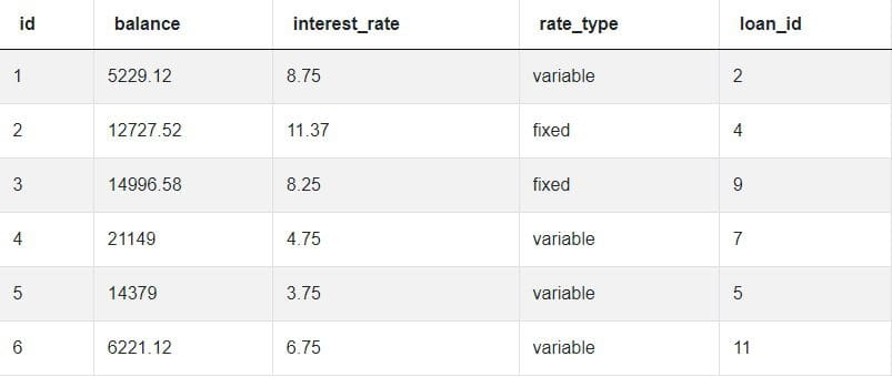
Let’s take a look at the loans table:
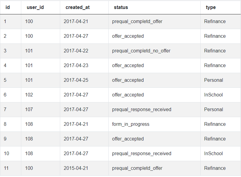
Next, the submissions table:
To answer this question successfully, it’s essential to analyze both tables and the data within them. Then we can use aggregate window functions to solve key pieces of the puzzle: find the most recent submission for each user.
To do this, a candidate must understand that the MAX() aggregate function will return the ‘highest’ date, which in SQL is equivalent to the latest date. MAX() window function must be applied to the created_at column in the loans table, where every record represents a single submission.
Another key piece of the puzzle is that the rows should be partitioned by user_id value, to make sure we generate the latest date for every unique user, in case they’ve made multiple submissions. The question specifies that we should find the latest submission of the ‘Refinance’ type, so our SQL query should include that condition.
Value Window Functions in SQL
SQL developers can use these functions to take values from other rows in the table. Like the other two types of window functions, there are five distinct functions of this kind. These are exclusively for window functions:
LAG() function allows us to access values from previous rows.
LEAD() is the opposite of LAG(), and allows us to access values from records that come after the current row.
FIRST_VALUE() function returns the first value from the dataset and allows us to set the condition for ordering the data, so the developer can control which value will come first.
The LAST_VALUE() function works the same way as the previous function, but it returns the last value instead of the first.
NTH_VALUE() function allows developers to specify which value in the order should be returned.
Time Series Analysis
Functions like LAG() and LEAD() allow you to extract values from the rows that follow or precede each row. For this reason, SQL developers often use them to work with time-series data, tracking daily or monthly growth, and other use-cases. Let’s look at a question asked at Amazon interviews that can be solved using the LAG() function.
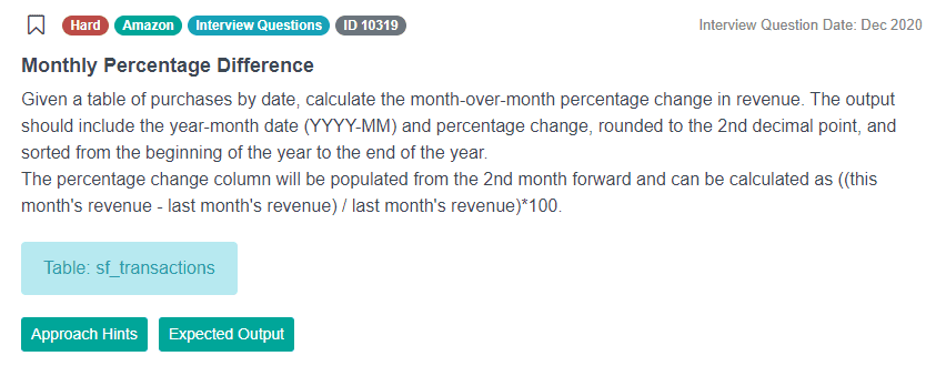
In this question, candidates have a fairly simple task: calculate monthly revenue growth based on the provided data. Ultimately, the output table should include a percentage value that represents month-over-month growth.
The LAG() window function allows us to solve this difficult question in just a few lines of code. Let’s take a look at the actual recommended solution:
SELECT to_char(created_at::date, 'YYYY-MM') AS year_month,
       round(((sum(value) - lag(sum(value), 1) OVER w) / (lag(sum(value), 1) OVER w)) * 100, 2) AS revenue_diff_pct
FROM sf_transactions
GROUP BY year_month WINDOW w AS (
                                 ORDER BY to_char(created_at::date, 'YYYY-MM'))
ORDER BY year_month ASC
The date values in the table are ordered from earlier to later. Therefore, all we have to do is calculate the total revenue for every month, and use the LAG() function to access the income value from the previous month and use it, along with current month’s revenue to calculate the monthly difference expressed in percentages.
In the solution above, we use the round() function to round the results of our equation. First, we define the window of data, where we arrange the date values and organize them in a specific format. We could do this directly in the window functions, but we will have to use it in multiple places. It’s more efficient to define the window once, and simply reference it as w.
First, by subtracting lag(sum(value), 1) from sum(value) we find the numerical difference between each month and its previous month (except for the first, which doesn’t have a previous month). We divide this number by the previous month’s revenue, which we find using the lag() function. Finally, we multiply the result by 100 to get the percentage value, and specify that the value needs to be rounded to two decimal points.
Final Words
It shouldn’t be a surprise that many interview questions test the candidate’s knowledge of SQL window functions. Employers know that to perform at the highest level, data scientists must understand this part of SQL very well.
If you aspire to the role where you’ll be writing advanced SQL queries, a thorough understanding of SQL window functions can help you find easy solutions to complicated problems.
Nate Rosidi is a data scientist and in product strategy. He's also an adjunct professor teaching analytics, and is the founder of StrataScratch, a platform helping data scientists prepare for their interviews with real interview questions from top companies. Connect with him on Twitter: StrataScratch or LinkedIn.