Visualizing Your Confusion Matrix in Scikit-learn
Defining model evaluation metrics is crucial in ensuring that the model performs precisely for the purpose it is built. Confusion Matrix is one of the most popular and effective tools to evaluate the performance of the trained ML model. In this post, you will learn how to visualize the confusion matrix and interpret its output.
Introduction
There are many machine learning algorithms packaged in the form of standard software to train your data. So, training and building an algorithm is trivial. But what separates an experienced data scientist from a novice is how they evaluate the quality of their machine learning model.
During the model development stage, you train a set of algorithms on the given data, evaluate their performance and eventually select the best-performing model. But how we define a metric to choose the best model out of the candidate set of algorithms plays a crucial role in the success of your machine learning solution.
Confusion Matrix
When we talk about a confusion matrix, it is always in the classification problem context. Let’s take an example of binary classification (two-class problem). Here we have binary or two states of a variable known as the target variable. The task is to predict the state given some attributes or independent variables.
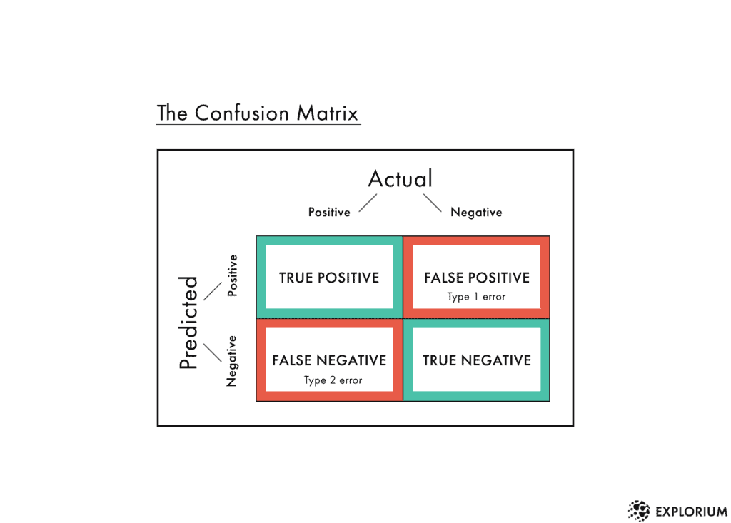
The four counts we get from the state interaction between the predicted states and the actual states are what form our confusion matrix.
Source: https://www.explorium.ai/wp-content/uploads/2019/07/Confusion-1024x733.png
Components of Confusion Matrix
The four quadrants are defined as True Negative (TN), True Positive (TP), False Positive (FP), False Negative (FN). If you are not acquainted with these terms and they look confusing going by their name, then stay tuned and read along, these terms are demystified in the section below:
True Negative: Whenever we say True, it means our predictions match the actuals. True Negative means both predictions and actuals are of a negative class.
True Positive: Similarly when predictions and actuals are of positive class, it’s called a True Positive.
Akin to the True categories explained above where the actuals and predictions are conforming, False categories indicate that prediction is not matching the ground truth i.e. actuals. This is the area of concern for data scientists. Optimistically speaking, this false section is also the key driver that enables data scientists to identify the limitations and concerns attributed to either the algorithmic model or the data itself. This process is called error analysis which puts focus on deviations of predictions from the actuals.
False Positive: When a prediction is positive and the actual is negative it’s called a False Positive.
False Negative: Similar to False Positive, False Negative is when the prediction is negative but the actual is positive.
The confusion matrix thus represents the count of all TP, TN, FP, and FN instances.
Understanding the Derived Metrics
The four numbers in a confusion matrix standalone give us an understanding of the model performance at a granular level but data scientists need one single measure that can help them evaluate the overall model performance. This helps them formulate an ML problem as a minimization problem. Hence, there are some key evaluation metrics derived from these four measures as explained below:
Accuracy: Accuracy is defined as all correctly predicted instances over all instances. Mathematically:
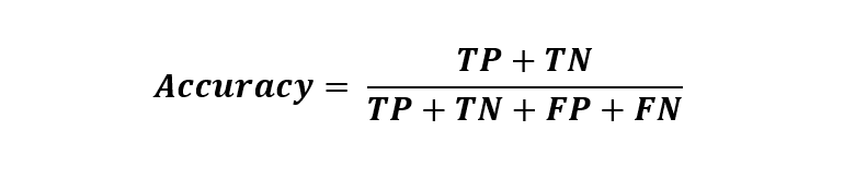
It is not a robust metric to go by especially when the data has a class imbalance. Class Imbalance is when one class dominates the other.
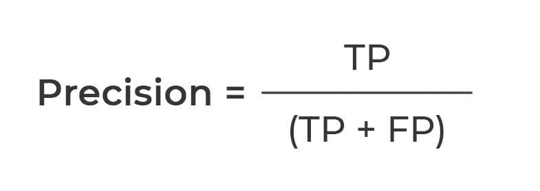
Precision: Precision measures the fraction of positive predictions matching the actuals. Mathematically:
Recall: Recall measures the fraction of positive instances correctly identified. Mathematically:

F1 or F-beta: While Precision tries to minimize FPs and Recall tries to minimize FNs, the F-1 metric maintains a balance between precision and recall and is defined as a harmonic mean between the two.
F-beta is a weighted harmonic mean of precision and recall. Mathematically it’s defined as:
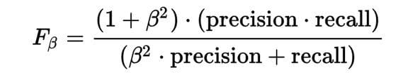
Where a β value less than 1 would lower the impact of Precision and vice-versa. At β=1, F-beta becomes F1.
Now that the metrics of a classification problem are under our belt. Let’s pick a dataset, train a model and evaluate its performance using a confusion matrix.
Scikit-learn Implementation
We will consider the heart-disease dataset from Kaggle for building a model to predict whether the patient is prone to heart disease or not. So, it is a case of binary classification where ‘heart disease’ is class 1 and ‘no heart disease’ is class 0.
Import Libraries
import pandas as pd
from sklearn.model_selection import train_test_split
from sklearn.tree import DecisionTreeClassifier
from sklearn.metrics import confusion_matrix, ConfusionMatrixDisplay
Read Data
df = pd.read_csv('heart.csv')
df.head()
Split train and test dataset
X = df[['age', 'sex', 'cp', 'trestbps', 'chol', 'fbs', 'restecg', 'thalach', 'exang', 'oldpeak', 'slope', 'ca', 'thal']]
y = df['target']
X_train, X_test, y_train, y_test = train_test_split(X, y, test_size=0.3, random_state=4
Train Model
clf = DecisionTreeClassifier()
clf.fit(X_train, y_train)
Evaluate predictions
y_pred = clf.predict(X_test)
cm = confusion_matrix(y_test, y_pred)
ConfusionMatrixDisplay(cm, clf.classes_).plot()
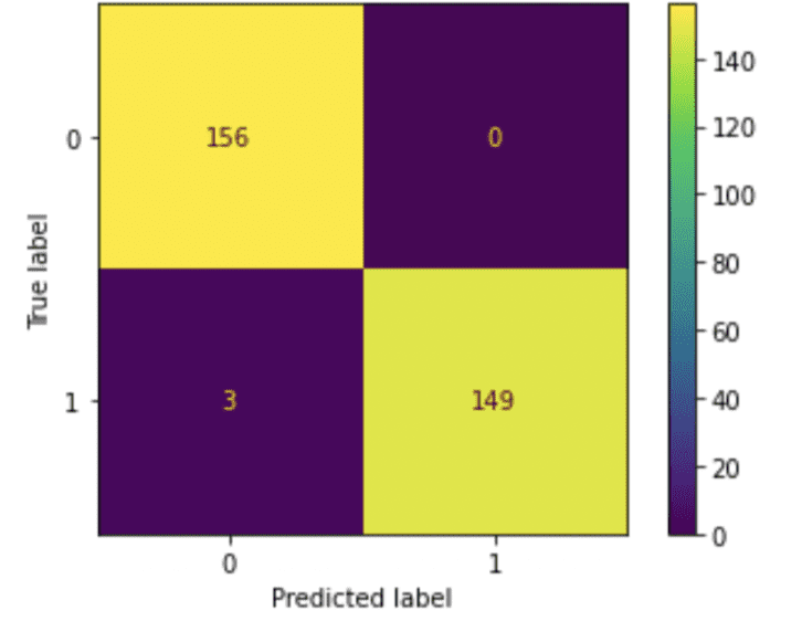
Interpreting Confusion Matrix and Computing Derived Metrics
From the above confusion matrix let’s get the four numbers:
- True Positives: 149 (when both Predicted and True labels are 1)
- True Negatives: 156 (when both Predicted and True labels are 1)
- False Positives: 0 (when both Predicted and True labels are 1)
- False Negatives: 3 (when both Predicted and True labels are 1)
Derived Metrics are computed using the mathematical expressions explained in the previous section:
- Accuracy: (156+149)/(156+149+0+3) = 99.03%
- Precision: 149/(149+0) = 100%
- Recall: 149/(149+3) = 98.03%
- F1: 2*149/(2*149+0+3) = 99%
Summary
In this post we understood the usage and importance of confusion matrix in a classification algorithm. We then learned the four measures of a confusion matrix and how can we compute the derived metrics along with their advantages and disadvantages. Further, the article illustrates how to display a confusion matrix with the help of an example of a binary classification problem. Hopefully, the post has helped you build an understanding of what are the various metrics to evaluate the model performance and which one to use when.
Vidhi Chugh is an award-winning AI/ML innovation leader and an AI Ethicist. She works at the intersection of data science, product, and research to deliver business value and insights. She is an advocate for data-centric science and a leading expert in data governance with a vision to build trustworthy AI solutions.