What are Moment-Generating Functions?
A brief overview of what moment-generating functions are and how they are used in probability and statistics.
Data science is a multidisciplinary field. As such, it often favors polyglots and polymaths. It requires an understanding of computational and applied maths, which can be off-putting for aspirational data scientists from a purely coding background. However, having a grasp of mathematical statistics is important, especially if you plan to create algorithms and data models for forecasting outcomes.
In most cases, the best way to learn anything is to break it down into concepts. This goes for concepts in probability and statistics too. Moment-generating functions (MGF) are one of these concepts all data scientists should know. The following guide will answer what they are and how you can implement them programmatically.
What are Moments in Probability and Statistics?
If you take the term moment-generating functions literally, what you can see is that MGFs are functions that generate moments. But what are moments? In statistics, we use what is known as a distribution to illustrate how values are spread in a field, i.e., which values are common and which ones are rare.
Data scientists and statisticians use moments to measure distributions. Fundamentally, moments are parameters of the distribution, and they can be used to determine or describe its shape, allowing you to extract information (metadata) about your data. We’ll look at the four most common moments below.
The Mean E(X)
The mean is the first moment. It describes the central location/position/tendency of a distribution. Additionally, it is the initial expected value and is also referred to as a (mathematical) expectation or average. In the cases where results have a joint probability of occurrence, we use the arithmetic mean formula:

In simpler terms, the sum of all variable values can be divided by the number of values [(Sum of values)÷(Total numbers of Values)].
However, if the results do not share the same probability of occurrence, you must calculate the outcome of each probability, sum up the values for the variable and then multiply it by the corresponding outcome/probability.
The mean formula is one of the most popular ways to measure the average or central tendency. It can also be represented as the median (middle value) or mode (the most likely value).
The Variance E(X^2)
The variance is the second moment. It indicates the width or spread of the distribution – how far the values are from the average or norm. This moment is ultimately used to illustrate or find any deviations in the distribution or data set. We typically use the standard deviation, which is represented by the square root of the variance [E(X^3)].
The Skewness E(X^3)
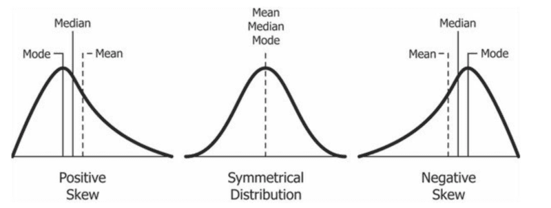
The skewness is the third moment. It indicates the asymmetry of the distribution or its lop-sidedness in relation to the distribution’s mean. The skewness affects the relationship between the mean median and mode. A distribution’s skewness can be represented in one of three categories:
- Symmetrical Distribution: Where both sides/tails of the distribution are symmetrical. In this category, the value of the skewness is 0. The mean, median, and mode are the same in a perfectly symmetrical (unimodal) distribution.
- Positively Skewed: Where the right side/tail of the distribution is longer than the left. This is used to identify and represent outliers with values greater than the mean. This category may also be referred to as skewed to the right, right-tailed, or right-skewed. Generally, the mean is greater than the median, which is greater than the mode (mode < median < mean).
- Negatively Skewed: Where the left side/tail of the distribution is longer than the right. We use it to identify and represent outliers whose values are lesser than the mean. This category can also be referred to as skewed to the left, left-skewed, or left-tailed. Generally, the mode is greater than the median, which is greater than the mean (mode > median > mean).
You can also use the following simple formulas to find the skewness:
or
Source: Creative Commons
Kurtosis E(X^4)
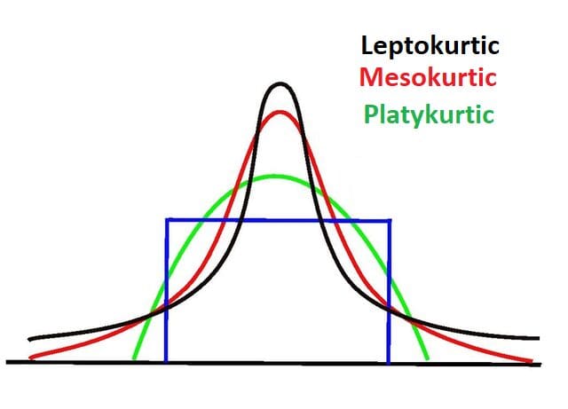
Kurtosis is the fourth moment. We use it to measure and indicate the occurrence of outliers by using the “tailedness” of the distribution. Thus, kurtosis is most concerned with the tails of the distribution. It helps us ascertain if the distribution is normal or filled with extreme values.
Generally, normal distributions have a kurtosis value of 3 or an excess kurtosis of 0. Distributions with this type of kurtosis are referred to as mesokurtic. A distribution with lighter tails and a kurtosis value lesser than three (K < 3) is referred to as having negative kurtosis. In these cases, the distribution is typically broad and flat and referred to as platykurtic.
On the other hand, a distribution with heavier tails and a kurtosis value greater than three (K > 3) is referred to as having a positive kurtosis. In these cases, the distribution is thin, has a pointed or high peak, and is referred to as leptokurtic. High kurtosis indicates that the distribution contains outliers.
Now that we’ve covered what moments are, we can discuss moment-generating functions (MGF).
What are Moment Generating Functions (MGF)?
Moment-generating functions are ultimately functions that allow you to generate moments. In the case where X is a random variable with a cumulative distribution function Fx and where the expected variable of t is in close proximity to some neighborhood of zero, the MGF of X is defined as:
Where X is discrete, and pi represents the probability mass function (PMF), the definition will be:
Where X is continuous and f(X) represents the probability density function (PDF), the definition will look like this:
In cases where we’re trying to find the raw moment, we must find the value of E[xn]. This involves using the nth derivative of E[etx]. We also simplify it by plugging in 0 as the value of t (t = 0):
Thus, finding the first raw moment (mean) using the MGF with t as 0 looks like this:
You can find the second raw moment using the same approach:
You can use Taylor’s Expansion (ex=1+x1!+x22!+x33!+…, -∞
Why are Moment-Generating Functions Necessary?
MGF offers an alternative to integrating the PDF in a continuous probability distribution to find its moments. In programming, searching for the right integration makes algorithms far more complex and requires more computing resources, increasing the load or run-time of the program. MGFs and their derivations are far more efficient at finding moments.
Conclusion
Finding the moments of a distribution without using an MGF is possible but calculating higher-order moments without using MGF gets complicated. Python’s built-in statistic module comes with a sufficient list of functions that can be used to calculate moments from a dataset. However, this isn’t the only option for working with statistical functions in Python.
The above guide provides a basic exploration of moments and moment-generating functions. As a programmer or data scientist, you may never have to manually calculate raw moments or try to derive central moments manually. In all likelihood, there are a variety of modules and libraries that do that for you. However, it’s always important to understand what goes on in the background.
Nahla Davies is a software developer and tech writer. Before devoting her work full time to technical writing, she managed — among other intriguing things — to serve as a lead programmer at an Inc. 5,000 experiential branding organization whose clients include Samsung, Time Warner, Netflix, and Sony.