By Diego Lopez Yse, Data Scientist
It is rare that you get data in exactly the right form you need it. Often you’ll need to create some new variables, rename existing ones, reorder the observations, or just drop registers in order to make data a little easier to work with.
This is called data wrangling (or preparation), and it is a key part of Data Science. Most of the time data you have can’t be used straight away for your analysis: it will usually require some manipulation and adaptation, especially if you need to aggregate other sources of data to the analysis.
In essence, raw data is messy (usually unusable at the start), and you’ll need to roll up your sleeves to get to the right place. For this reason, all the activity you take to make it “neat” enough is as important as the algorithms you choose to work with. In almost all cases, the data-wrangling piece is a prerequisite to the math/modelling and a majority of the time is spent on cleaning the data in a real-world scenario.
Let’s face it: data won’t be ready or able to be consumed by any algorithm without extra effort.
So, let’s discuss some concepts that will help you face this sometimes seemingly titanic task. In practical terms, datasets can be considered as tables composed of variables (columns), and observations (rows):
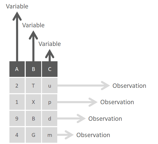
Columns or variables should be all of the same type (e.g. numeric, date, character, etc), while rows or observations (also referred to as “vectors”) can be a mixture of all types of data.
So, to begin discussing data preparation we need to distinguish between data wrangling for one, and more than one datasets.
Single Dataset
The main tasks to deal with single datasets are:
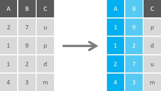
Sort (Arrange)
One of the most basic functions of data wrangling is to order rows by the value or characters of a variable, or a selection of them. This can be in alphabetical order, from the smallest to highest number, or others.
In most cases, you’ll need to sort one single variable, but sorting can be done with multiple criteria, by defining one main parameter and then the subsequent ones.
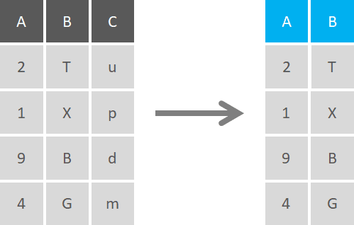
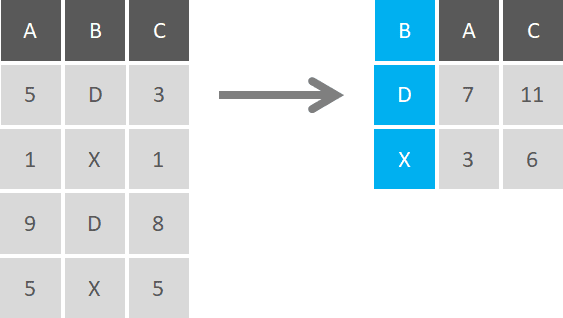
Select
Selection is the activity of choosing columns in a dataset based on a defined criteria. This can be as simple as picking a column based on its name or position, or using different statements on a range of columns. It’s possible to make partial matching on columns by using statements like “starts with”, ends with”, or “contains” in the selection statement, or even exclude a specific column (or a chunk of columns) from the selection.
You can use conditional selections to show columns that meet certain criteria, like showing only columns that contain numeric data, or character data for example. The other way around, you can select the negation of these conditions, and select only data that doesn’t meet one or more conditions(e.g. show only data that’s not date formatted).
Additionally, you can use logical expressions on numeric data like selecting values that are above a certain threshold or contain an average value below a certain parameter.
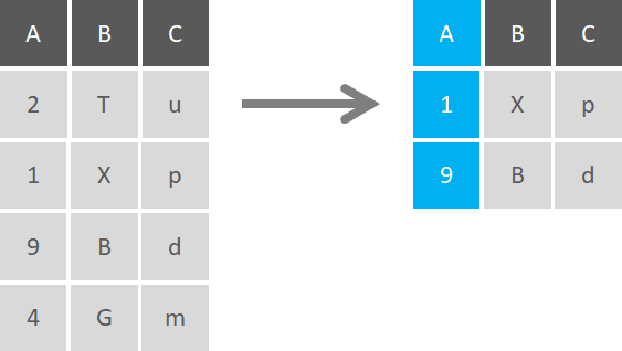
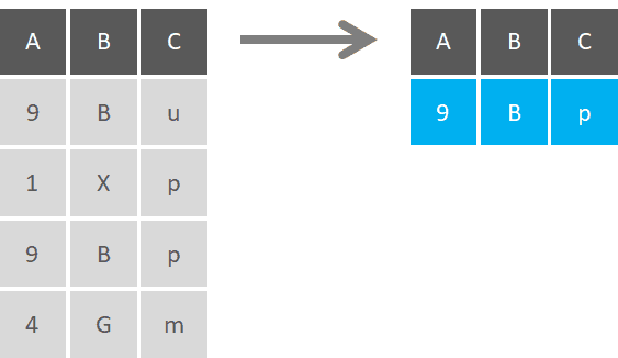
Filter
When you don’t want to include all rows of a dataset in your analysis, you can use a filter function to return rows that match 1 or more conditions. This is a sub-setting procedure that allows you to pick specific values by column/s, a range of values, or even approximations with ranges of tolerance. With characters, you can filter to include or exclude results based on exact or partial character matches, and also find registers that begin with, end up or contain certain terms.
Filters with multiple conditions can be combined with AND, OR, and NOT conditions, and you can even specify to return values when only one condition out of two is met, but not doing it when both are met.
Similar to selection functions, filters can be applied to all columns with no discrimination, or used with conditions to return just the registers that meet them. Filter functions are especially useful to filter out NA or missing values rows. You can also filter the top highest or lowest values and show only those registers, without the need to show the whole dataset rows.
Filtering is the right method for getting the unique or distinct values in a data frame, or just counting the number of them.
Aggregate
Data aggregation is the process of gathering information and expressing it in a summary form, with the objective of performing statistical analysis (summarizing) or creating particular groups based on specific variables (grouping by).
- Summarize
Summarized operations use a single numerical value to condense a large number of values, for example, the mean/average or the median. Other examples of summary statistics include the sum, the smallest (minimum) value, the largest (maximum) value, and the standard deviation: these are all summaries of a large number of values. This way, a single number gives insights into the nature of a potentially large dataset, just by computing aggregations.
Summarizing can be conditional, where you state the arguments prior to performing the operation. For example, if you consider calculating the mean of all variables, you can define a condition to do so only for variables that are numeric, since categorical variables will produce an error (they have no mean).
- Group by
In most cases, we don’t just want to summarize the whole data table, but we want to get summaries by groups, which gives better information on the distribution of the data. To do this, you first need to specify by which variable(s) you want to divide the data, and then summarize those categories.
Group by is a classic aggregation function, that becomes powerful when combined with a summarize function. You can group by multiple variables, and then summarize multiple variables at the same time, which is quite useful when you want to brake down variables by categories. This approach is also known as the “Split-Apply-Combine Principle”, in which you break up a big problem into small manageable pieces (Split), operate on each piece independently (Apply), and then put all the pieces back together (Combine).

Transform
Transforming data involves the creation of new record fields through existing values in the dataset, and is one of the most important aspects of data preparation . It’s not easy to identify when (and if) data transformations are required, and it’s even more complex to define the type of transformation required.
But why would you bother transforming a variable? You may transform categorical variables to a format which will better work for classification and regression models, or use logarithmic transformations to transform non-linear models into linear models and work with skewed data.
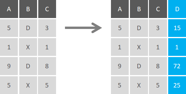
You can perform all types of transformations (e.g. standardization, normalization, or binarization), and apply the same transformation to multiple variables. You can concatenate variables to create new ones, or perform basic arithmetic operations to create them.
Replace
This is what you use when you want to convert specific characters to something else. You can convert numerical characters to data & time formats, or re-code variables to fit models. This technique is typically used to replace missing values, although we’ll deep dive in that matter later.
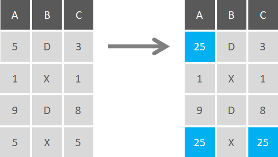
The main differences between Transformation and Replacement is that you’re not creating additional variables or registers (you’re modifying existing ones), and you can change the nature of the variable (e.g. change a character variable to a numerical code), without creating new record fields. You can perform replacements on all variables, set conditions for them, or do it just on specific registers.
Combining Datasets
The true power of Data Science comes with data volume. In reality, data are hosted on different servers and exist in many different files. When the data you need come from multiple sources, it’s essential to know how to combine them. Let’s explore some techniques generally used to exploit this matter:
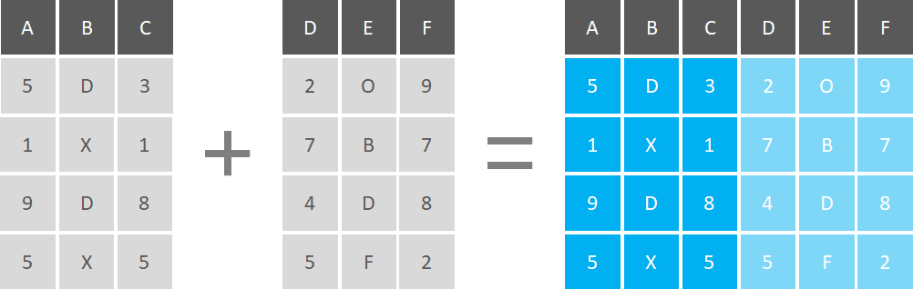
Concatenate
In general, you can add information by adding more rows or by adding more columns to your dataset. When you have datasets that have the same set of columns (variables) or have the same set of rows (observations), you can concatenate or bind them vertically or horizontally, respectively.

If you’re going to add more rows, datasets must have the same set of variables (columns), but observations don’t have to be in the same order.
If you’re going to add more columns, you should check that the quantity and the order of the observations are the same.
It’s important to note that if you have the same observation across multiple datasets and you concatenate them vertically, you'll end up with duplicate observations in your table.
Merge
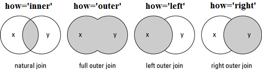
Joins are the standard way to merge datasets into a single table. A Join is used to combine rows from two or more datasets, based on a related column between them. There are many types of joins, being the main ones:
- Inner Join: produces only the set of records that match in both datasets. In programming logic, you can think in terms of AND.
- Full Outer Join: produces the set of all records in both datasets, with matching records from both sides where available. If there is no match, the missing side will contain NULL values.
- Left Join: produces a complete set of records from table x, with the matching records (where available) in Table y. If there is no match, the right side will contain NULL values.
- Right Join: returns all the records from table y and also those records which satisfy a condition from table x. If there is no match, the output or the result-set will contain the NULL values.
You can find examples in Python in this link
Missing Values
Often encoded as NaNs or blanks, missing data (or missing values) is defined as the data value that is not stored for a variable in the observation of interest. The problem of missing data is relatively common in almost all research and can have a significant effect on the conclusions that can be drawn from the data. Missing values can be categorized into:
- Missing completely at random (MCAR): when the probability that the data are missing is not related to either the specific value which is supposed to be obtained or the set of observed responses. This is the case of data that is missing by design (e.g. because of an equipment failure).
- Missing at random (MAR): when the probability that the responses are missing depends on the set of observed responses, but is not related to the specific missing values which are expected to be obtained.
- Missing not at random (MNAR): the only way to obtain an unbiased estimate of the parameters in such a case is to model the missing data (e.g. people with high salaries that generally don’t reveal their incomes in surveys)
There are many strategies for dealing with missing data, and none of them are applicable universally. Resolving this issue require both experience and domain based, and it starts by understanding the nature of the missing value.
Some commonly used methods for dealing with this problem include:
- dropping instances with missing values
- dropping attributes with missing values
- imputing the attribute (e.g. mean, median or mode) for all missing values
- imputing the attribute missing values via linear regression
- Last observation carried forward
You can also develop your own strategy, like dropping any instances with more than 2 missing values and use the mean attribute value imputation those which remain. Or what’s even more complex, build a Decision Tree to fill those missing values.
Outliers
An outlier is an observation that lies at an abnormal distance from other values, diverging from otherwise well-structured data. They are data points that don’t belong to a certain population.
In order to identify them it’s essential to perform Exploratory Data Analysis (EDA), examining the data to detect unusual observations, since they can impact the results of our analysis and statistical modeling in a drastic way. Look at the following example:

Do you see how these outliers modify the slope of the regression on the left? Which of the 2 regression lines better represent the dataset?
All right, so you find an outlier, remove it, and move on with your analysis. NO! Simply removing outliers from your data without considering how they’ll impact the results is a recipe for disaster.
Outliers aren’t necessarily a bad thing
This is where your judgment comes to play. Outliers can drastically bias/change the fit estimate and prediction of your model, but they need to be trated carefully. Detecting outliers is one of the core problems in disciplines like Data Science, and the way you deal with them will affect your analysis and model performance. Some common ways to detect outliers are:
- Z-Score: is a metric that indicates how many standard deviations a data point is from the sample’s mean, assuming a gaussian distribution. The intuition behind Z-score is to describe any data point by finding their relationship with the standard deviation and mean of the group of data points. This way, we re-scale and center the data and look for data points which are too far from zero. These data points which are way too far from zero will be treated as the outliers (in most of the cases a threshold of 3 or -3 is used).
- Interquartile Range (IQR) Score: is a measure of statistical dispersion, being equal to the difference between 75th and 25th percentiles, or between upper and lower quartiles, IQR = Q3 − Q1. It is a measure of the dispersion similar to standard deviation or variance, but is much more robust against outliers.
- DBSCAN algorithm: is a density-based clustering. Although not an outlier detection method per-se, it grows clusters based on a distance measure. DBSCAN calculates the distance between points (the Euclidean distance or some other distance) and looks for points which are far away from others: points that do not belong to any cluster get their own class: -1.
Outliers can be of two types: Univariate and Multivariate. Univariate outliers can be found when we look at distribution of a single variable, while multi-variate outliers are outliers in an n-dimensional space: in order to find them, you have to look at distributions in multi-dimensions.
Similarly to missing values, outliers can be imputed (e.g. with mean / median / mode), capped (replacing those outside certain limits), or replaced by missing values and predicted.
Feature Scaling
The range of the variables in your dataset may differ significantly. Some features may be expressed in kilograms while others in grams, another might be liters, and so on. Using the original scale may put more weights on variables with a large range, and that can be a problem. Feature scaling is a method to unify self-variables or feature ranges in data.
Some distanced-based algorithms like K-Nearest-Neighbours, SVMs or Neural Networks can be affected when the range of the features is very different (features with large range will have a high influence in computing the distance). On the other hand, if an algorithm is not distance-based (e.g. Naive Bayes or Decision Trees), feature scaling won’t have an impact.
So, how to do you scale?
- Normalization: is a scaling technique in which values are shifted and rescaled so that they end up ranging between 0 and 1.
- Standardization: re-scales a feature value so that it has distribution with 0 mean value and variance equals to 1.
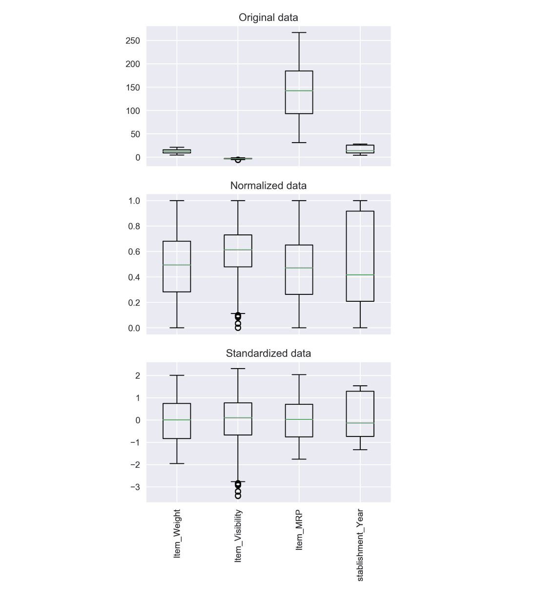
The choice of using normalization or standardization will depend on the problem and the machine learning algorithm. There is no universal rule to use one or the other, so you can always start by fitting your model to raw, normalized and standardized data and compare the performance for best results.
Feature scaling can improve the performance of some machine learning algorithms significantly but have no effect on others.
Encoding
Many machine learning algorithms can support categorical values without further manipulation but there are many more algorithms that do not. Categorical variables can only take on a limited, and usually fixed, number of possible values. Some examples include color (“Red”, “Yellow”, “Blue”), size (“Small”, “Medium”, “Large”) or geographic designations (State or Country).
Again, there is no single answer on how to approach this problem, but let’s present some of the main strategies:
- Replace values: involves replacing the categories with the desired numbers. This is the simplest form of encoding where each value is converted to an integer, and is particularly useful for ordinal variable where the order of categories is important.
- Label encoding: transforms non-numerical labels into numerical labels. Each category is assigned a unique label starting from 0 and going on till n_categories — 1 per feature. Label encoders are suitable for encoding variables where alphabetical alignment or numerical value of labels is important, but have the disadvantage that the numerical values can be misinterpreted by the algorithm: should the variable encoded as 5 be given 5x more weight than the one encoded as 1?
- One-Hot encoding: involves converting each category value into a new column and assign a “1” or “0” (true/false) value to the column. This has the benefit of not weighting a value improperly, but it’s not very efficient when there are many categories, as that will result in formation of as many new columns.
- Binary encoding: first encodes the categories as ordinal, then those integers are converted into binary code, and the digits from that binary string are split into separate columns. This is good for high cardinality data as it creates very few new columns: most similar values overlap with each other across many of the new columns, allowing many machine learning algorithms to learn the similarity of the values.
Besides these strategies, there are multiple other approaches to encoding variables, so it’s important to understand the various options and how to implement them on your own data sets.
You can find a complete tutorial for encoding in Python here.
Dimensionality Reduction
As data volume increases, this can have a significant impact on the time of implementation of certain algorithms, make visualization extremely challenging, and even make some machine learning models useless. Statistically, the more variables we have, the more number of samples we will need to have all combinations of feature values well represented in our sample.
Dimensionality reduction is the process of reducing the total number of variables in our data set in order to avoid these pitfalls. The concept behind this is that high-dimensional data are dominated “superficially” by a small number of simple variables. This way, we can find a subset of the variables to represent the same level of information in the data or transform the variables to a new set of variables without losing much information.
Probably the 2 main common approaches to deal with high-dimensional data are:
- Principal Component Analysis (PCA): is probably the most popular technique when we think of dimension reduction. The idea is to reduce the dimensionality of a dataset consisting of a large number of related variables while retaining as much variance in the data as possible. PCA is an unsupervised algorithm that creates linear combinations of the original features. A principal component is a linear combination of the original variables and works in the following way: principal components are extracted in such a way that the first principal component explains maximum variance in the dataset. The second principal component tries to explain the remaining variance in the dataset and is uncorrelated to the first principal component. The third principal component tries to explain the variance which is not explained by the first two principal components and so on. This way, you can reduce dimensionality by limiting the number of principal components to keep based on cumulative explained variance. For example, you might decide to keep only as many principal components as needed to reach a cumulative explained variance of 90%.

- Linear Discriminant Analysis (LDA): unlike PCA, LDA doesn’t maximize explained variance: it maximizes the separability between classes. It seeks to preserve as much discriminatory power as possible for the dependent variable, while projecting the original data matrix onto a lower-dimensional space: it projects data in a way that the class separability is maximized. LDA is a supervised method that can only be used with labeled data. Examples from same class are put closely together by the projection. Examples from different classes are placed far apart by the projection. It’s important to note that LDA does make some assumptions about our data. In particular, it assumes that the data for our classes are normally distributed (Gaussian distribution).
You can find a full implementation of both methods in Python here.
Conclusion
In real world, data comes split across multiple datasets and across many different formats. Whether you like it or not, you’ll need to face some of the problems we described, and the better you prepare, the less you’ll suffer.
The important thing to remember is that there’s no free lunch. To solve a problem you need to make a decision, and that decision will bring consequences. When you drop missing values or remove outliers with percentiles, you’re changing the dataset. Even when you change the smallest thing (which you’ll need to do), you’re changing your raw data. That’s fine, no need to worry, but keep in mind that your actions (big or small) carry out consequences.
Interested in these topics? Follow me on Linkedin or Twitter
Bio: Diego Lopez Yse is an experienced professional with a solid international background acquired in different industries (capital markets, biotechnology, software, consultancy, government, agriculture). Always a team member. Skilled in Business Management, Analytics, Finance, Risk, Project Management and Commercial Operations. MS in Data Science and Corporate Finance.
Original. Reposted with permission.
Related:
- 7 Steps to Mastering Data Preparation for Machine Learning with Python — 2019 Edition
- Time Complexity: How to measure the efficiency of algorithms
- Fantastic Four of Data Science Project Preparation