 7 Steps to Mastering Data Preparation for Machine Learning with Python — 2019 Edition
 7 Steps to Mastering Data Preparation for Machine Learning with Python — 2019 Edition
Interested in mastering data preparation with Python? Follow these 7 steps which cover the concepts, the individual tasks, as well as different approaches to tackling the entire process from within the Python ecosystem.
Interested in mastering data preparation with Python?
Data preparation, cleaning, pre-processing, cleansing, wrangling. Whatever term you choose, they refer to a roughly related set of pre-modeling data activities in the machine learning, data mining, and data science communities.
Wikipedia defines data cleansing as:
...is the process of detecting and correcting (or removing) corrupt or inaccurate records from a record set, table, or database and refers to identifying incomplete, incorrect, inaccurate or irrelevant parts of the data and then replacing, modifying, or deleting the dirty or coarse data. Data cleansing may be performed interactively with data wrangling tools, or as batch processing through scripting.
Data wrangling, for comparison, is defined by Wikipedia as:
...the process of manually converting or mapping data from one "raw" form into another format that allows for more convenient consumption of the data with the help of semi-automated tools. This may include further munging, data visualization, data aggregation, training a statistical model, as well as many other potential uses. Data munging as a process typically follows a set of general steps which begin with extracting the data in a raw form from the data source, "munging" the raw data using algorithms (e.g. sorting) or parsing the data into predefined data structures, and finally depositing the resulting content into a data sink for storage and future use.
I would say that it is "identifying incomplete, incorrect, inaccurate or irrelevant parts of the data and then replacing, modifying, or deleting the dirty or coarse data" in the context of "mapping data from one 'raw' form into another..." all the way up to "training a statistical model" which I like to think of data preparation as encompassing, or "everything from data sourcing right up to, but not including, model building." That is the vague-yet-oddly-precise definition we'll move forward with.
This article will update a previous version from 2017, in order to freshen up some of the materials throughout. I have tried to select a quality tutorial or two, along with video when appropriate, as a good representation of the particular lesson in each step.
Keep in mind that the article covers one particular set of data preparation techniques, and additional, or completely different, techniques may be used in a given circumstance, based on requirements. You should find that the prescription held herein is one which is both orthodox and general in approach.
Grab a snack and sit back, as we learn to master data preparation with Python.
Step 1: Preparing for the Preparation
First, let's stress what everyone else has already told you: it could be argued that this data preparation phase is not a preliminary step prior to a machine learning task, but actually an integral component (or even a majority) of what a typical machine learning task would encompass. For our purposes, however, we will separate the data preparation from the modeling as its own regimen.
As Python is the ecosystem in which we will be immersed, the following resources are a good jumping off point to ensure appropriate familiarity.
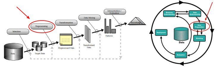
Data preparation can be seen in the CRISP-DM model (though it can be reasonably argued that "data understanding" falls within our definition as well). We can also equate our data preparation with the framework of the KDD Process — specifically the first 3 major steps — which are selection, preprocessing, and transformation. We can break these down into finer granularity, but at a macro level, these steps of the KDD Process encompass what data wrangling is.
While readers should be able to follow this guide with few additional resources, for those interested in a more holistic take on Pandas (likely the most important data preparation library in the Python ecosystem), helpful information can be found in the following:
- Intro to pandas data structures, by Greg Reda
- Modern Pandas (in 7 parts), by Tom Augspurger
Finally, for some feedback on the data preparation process from 3 insiders — Sebastian Raschka, Clare Bernard, and Joe Boutros — read this interview on Data Preparation Tips, Tricks, and Tools: An Interview with the Insiders before moving on.
Step 2: Exploratory Data Analysis
Exploratory data analysis (EDA) is an integral aspect of any greater data analysis, data science, or machine learning project. Understanding data before working with it isn't just a pretty good idea, it is a priority if you plan on accomplishing anything of consequence. Andrew Andrade concisely describes EDA as follows.
The purpose of EDA is to use summary statistics and visualizations to better understand data, and find clues about the tendencies of the data, its quality and to formulate assumptions and the hypothesis of our analysis.
The basic gist is that we need to know the makeup of our data before we can effectively select predictive algorithms or map out the remaining steps of our data preparation. Throwing our dataset at the hottest algorithm and hoping for the best is not a strategy.
To gain some intuition, watch this video by Prof. Patrick Meyer of the University of Virginia which provides an overview of EDA.
Then read Andrade's article on Exploratory data analysis, which provides additional details on how to go about EDA, and what its practical benefits are.
For a Python based approach tutorial on EDA, check out the article Exploratory Data Analysis (EDA) and Data Visualization with Python by Vigneshwer Dhinakaran, which actually goes a bit beyond traditional EDA in my view, and will introduce you to some of the additional concepts covered later in this article.
A library which dramatically shortens the code you need to write to perform EDA is Pandas Profiling, which creates HTML reports from Pandas DataFrames.
Generates profile reports from a pandas
DataFrame. The pandasdf.describe()function is great but a little basic for serious exploratory data analysis.pandas_profilingextends the pandas DataFrame withdf.profile_report()for quick data analysis.
You can run Pandas Profiling interactively in Jupyter notebooks with a single line of code:
df.profile_report()
Read the project's GitHub Readme for more information, and give it a try for yourself.
Step 3: Missing Values
There are many strategies for dealing with missing data, none of which are applicable universally. Some people will say "never use instances which include empty values." Others will argue "never use an attribute's mean value to replace missing values." Conversely, you may hear more complex methods endorsed wholesale, such as "only first clustering a dataset into the number of known classes and then using intra-cluster regression to calculate missing values is valid."
Listen to none of this. "Never" and "only" and other inflexible assertions hold no value in the nuanced world of data finessing; different types of data and processes suggest different best practices for dealing with missing values. However, since this type of knowledge is both experience and domain based, we will focus on the more basic strategies which can be employed.
Some commonly used methods for dealing with missing values include:
- dropping instances with missing values
- dropping attributes with missing values
- imputing the attribute { mean | median | mode } for all missing values
- imputing the attribute missing values via linear regression
Combination strategies may also be employed: drop any instances with more than 2 missing values and use the mean attribute value imputation those which remain. Clearly the type of modeling methods being employed will have an effect on your decision — for example, decision trees are not amenable to missing values. Additionally, you could technically entertain any statistical method you could think of for determining missing values from the dataset, but the listed approaches are tried, tested, and commonly used.
Since we are focusing on the Python ecosystem, from the Pandas user guide you can read more about Working with missing data, as well as reference the API documentation on the Pandas DataFrame object's fillna() function.
There are a lot of ways to accomplish filling missing values in a Pandas DataFrame. Here are a few basic examples:
You can also watch this video from codebasics on handling missing values with Pandas.
Step 4: Outliers
This is not a tutorial on drafting a strategy to deal with outliers in your data when modeling; there are times when including outliers in modeling is appropriate, and there are times when they are not (regardless of what anyone tries to tell you). This is situation-dependent, and no one can make sweeping assertions as to whether your situation belongs in column A or column B.
Outliers can be the result of poor data collection, or they can be genuinely good, anomalous data. These are 2 different scenarios, and must be approached differently, and so no "one size fits all" advice is applicable here, similar to that of dealing with missing values. A particularly good point of insights from the Analysis Factor article from above is as follows:
One option is to try a transformation. Square root and log transformations both pull in high numbers. This can make assumptions work better if the outlier is a dependent variable and can reduce the impact of a single point if the outlier is an independent variable.
Read this discussion, Outliers: To Drop or Not to Drop on The Analysis Factor, and the discussion Is it OK to remove outliers from data? on Stack Exchange, for further insight into this issue.
You can have a look at Removing Outliers Using Standard Deviation with Python as a simple example of removing outliers with Python. Then read this Stack Overflow discussion, Remove Outliers in Pandas DataFrame using Percentiles.
In the end, the decision as to whether or not to remove outliers will be task-dependent, and the reasoning and decision will be much more of a concern than the technical approach to doing so.
Step 5: Imbalanced Data
So, what if your otherwise robust dataset is made up of 2 classes: one which includes 95 percent of the instances, and the other which includes a mere 5 percent? Or worse, 99.8 vs 0.2 percent?

If so, your dataset is imbalanced, at least as far as the classes are concerned. This can be problematic, in ways which I'm sure do not need to be pointed out. But no need to to toss the data to the side yet; there are, of course, strategies for dealing with this.
A good explanation of why we can run into imbalanced data, and why we can do so in some domains much more frequently than in others (from 7 Techniques to Handle Imbalanced Data, below):
Data used in these areas often have less than 1% of rare, but “interesting” events (e.g. fraudsters using credit cards, user clicking advertisement or corrupted server scanning its network). However, most machine learning algorithms do not work very well with imbalanced datasets. The following seven techniques can help you, to train a classifier to detect the abnormal class.
Note that, while this may not genuinely be a data preparation task, such a dataset characteristic will make itself known early in the data preparation stage (the importance of EDA), and the validity of such data can certainly be assessed preliminarily during this preparation stage.
Tom Fawcett discusses this in his article Learning from Imbalanced Classes. Read it to get a better idea of the issue.
Then read this article, 7 Techniques to Handle Imbalanced Data by Ye Wu & Rick Radewagen, which covers techniques for handling class imbalance.
Step 6: Data Transformations
Wikipedia defines data transformation as:
In statistics, data transformation is the application of a deterministic mathematical function to each point in a data set — that is, each data point zi is replaced with the transformed value yi = f(zi), where f is a function. Transforms are usually applied so that the data appear to more closely meet the assumptions of a statistical inference procedure that is to be applied, or to improve the interpretability or appearance of graphs.
Transforming data is one of the most important aspects of data preparation, requiring more finesse than some others. When missing values manifest themselves in data, they are generally easy to find, and can be dealt with by one of the common methods outlined above — or by more complex measures gained from insight over time in a domain. However, when and if data transformations are required is often not as easily identifiable, to say nothing of the type of transformation required.
Let's look at a few specific transformations in order to get a better handle on them.
First, this overview of Preprocessing data from Scikit-learn's documentation gives some rationale for some of the most important preprocessing transformations, namely standardization, normalization, binarization, and a few others.
Standardization and normalization are a pair of often employed data transformations in machine learning projects. Both are data scaling methods: standardization refers to scaling the data to have a mean of 0 and a standard deviation of 1; normalization refers to the scaling the data values to fit into a predetermined range, generally between 0 and 1. Read this article by Shay Geller, Normalization vs Standardization — Quantitative analysis, to understand how the transformations work, how to perform them in the Python ecosystem, and gain some insight into best practice from the author.
One-hot encoding is a method for transforming categorical features to a format which will better work for classification and regression. Watch this video on one-hot encoding to gain a better understanding of how it does so, and see how it can be accomplished with Python tools.
Logarithmic distribution transformation is useful for transforming non-linear models into linear models and working with skewed data. Read this Stack Exchange discussion, When (and why) should you take the log of a distribution (of numbers)?, for the intuition. You can also have a look at this short tutorial from Data Science Made Simple, Log and natural Logarithmic value of a column in pandas python, for a quick overview of using Numpy to accomplish the transformation in Python.
This short tutorial from Ontario Tech University, Introduction to Exponential and Logarithmic Functions, takes a mathematical approach to explaining logarithmic and exponential transformations, along with visualizations, and can add to your intuition of what is happening to underlying data distributions when these transformations are performed. There are 3 pages in the tutorial, with the third having 2 videos which help drive the point home.
There are numerous additional standard data transformations which are regularly employed, depending on the data and your requirements. Experience with data preprocessing and preparation should provide intuition on what types of transformations are required in which circumstance.
Step 7: Finishing Touches & Moving Ahead
Alright. Your data is "clean." But what do you do with it?
If you want to go right to feeding your data into a machine learning algorithm in order to attempt building a model, you probably need your data in a more appropriate representation. In the Python ecosystem, that would generally be a Numpy ndarray (or matrix). This Stack Overflow discussion, Turning a Pandas Dataframe to an array and evaluate Multiple Linear Regression Model, can give some preliminary ideas on getting there.
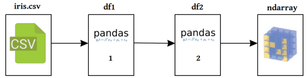
Note that most of our data preparation was performed in a combination of Pandas and Numpy in the preceding text; however, Pandas sits atop Numpy, and so learning how to manipulate the underlying Numpy matrix directly is a useful skill. Learn a bit more about that here.
What if you aren't quite ready to model the data yet, and instead want to store your clean Pandas DataFrame for later use? Quick HDF5 with Pandas by Giuseppe Vettigli will show you one such way to do so.
Once you have clean data in a proper representation for machine learning in Python, why not get right to the machine learning? First you will want to read 7 Steps to Mastering Basic Machine Learning with Python — 2019 Edition to gain an introductory understanding of machine learning in the Python ecosystem. Follow that up with 7 Steps to Mastering Intermediate Machine Learning with Python — 2019 Edition to enhance your knowledge (and be on the look out for an "advanced" installment as well).
For some differing viewpoints on data preparation, have a look at these:
- Tidying Data in Python, by Jean-Nicholas Hould
- Doing Data Science: A Kaggle Walkthrough Part 3 – Cleaning Data, by Brett Romero
- Machine Learning Workflows in Python from Scratch Part 1: Data Preparation
Note that this entire discussion is also fully and intentionally skipping any mention of feature selection for a specific reason: it deserves far more than a simple few sentences in this much more broad discussion. Be on the lookout for a similar guide for feature selection.
Related:
- 7 Steps to Mastering Basic Machine Learning with Python — 2019 Edition
- 7 Steps to Mastering Intermediate Machine Learning with Python — 2019 Edition
- 7 Steps to Mastering SQL for Data Science — 2019 Edition