Clustering with scikit-learn: A Tutorial on Unsupervised Learning
Clustering in machine learning with Python: algorithms, evaluation metrics, real-life applications, and more.
Image by Author
Clustering is a popular unsupervised machine learning technique, meaning it is used for datasets where the target variable or outcome variable is not provided.
In unsupervised learning, algorithms are tasked with catching the patterns and relationships within data without any pre-existing knowledge or guidance.
What does clustering do? It groups similar data points, enabling us to discover hidden patterns and relationships within our data.
In this article, we will explore the different clustering algorithms available and their respective use cases, along with important evaluation metrics to assess the quality of clustering results.
We will also demonstrate how to develop multiple clustering algorithms at once using the popular Python library scikit-learn.
Finally, we will highlight some of the most famous real-life applications that used clustering, discussing the algorithms used and the evaluation metrics employed.
But first, let’s get familiar with the clustering algorithms.
What are the Clustering Algorithms?
Below you will find an overview of the clustering algorithms and short definitions.
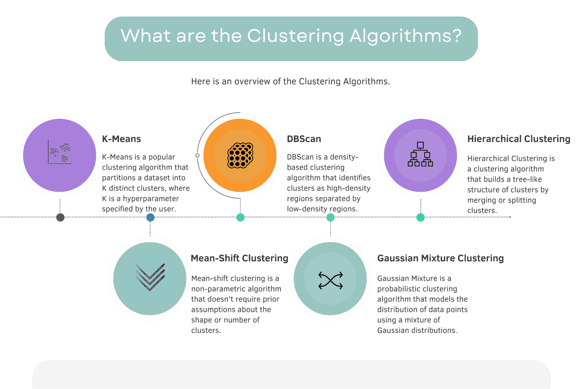
Image by Author
According to scikit-learn official documentation, there are 11 different clustering algorithms: K-Means, Affinity propagation, Mean Shift, Special Clustering, Hierarchical Clustering, Agglomerative Clustering, DBScan, Optics, Gaussian Mixture, Birch, Bisecting K-Means.
Here you can find the official documentation.
This section will explore the 5 most famous and important clustering algorithms. They are K-Means, Mean-Shift, DBScan, Gaussian Mixture, and Hierarchical Clustering.
Before diving deeper, let’s look at the following graph. It shows how these five algorithms work on six differently structured datasets.
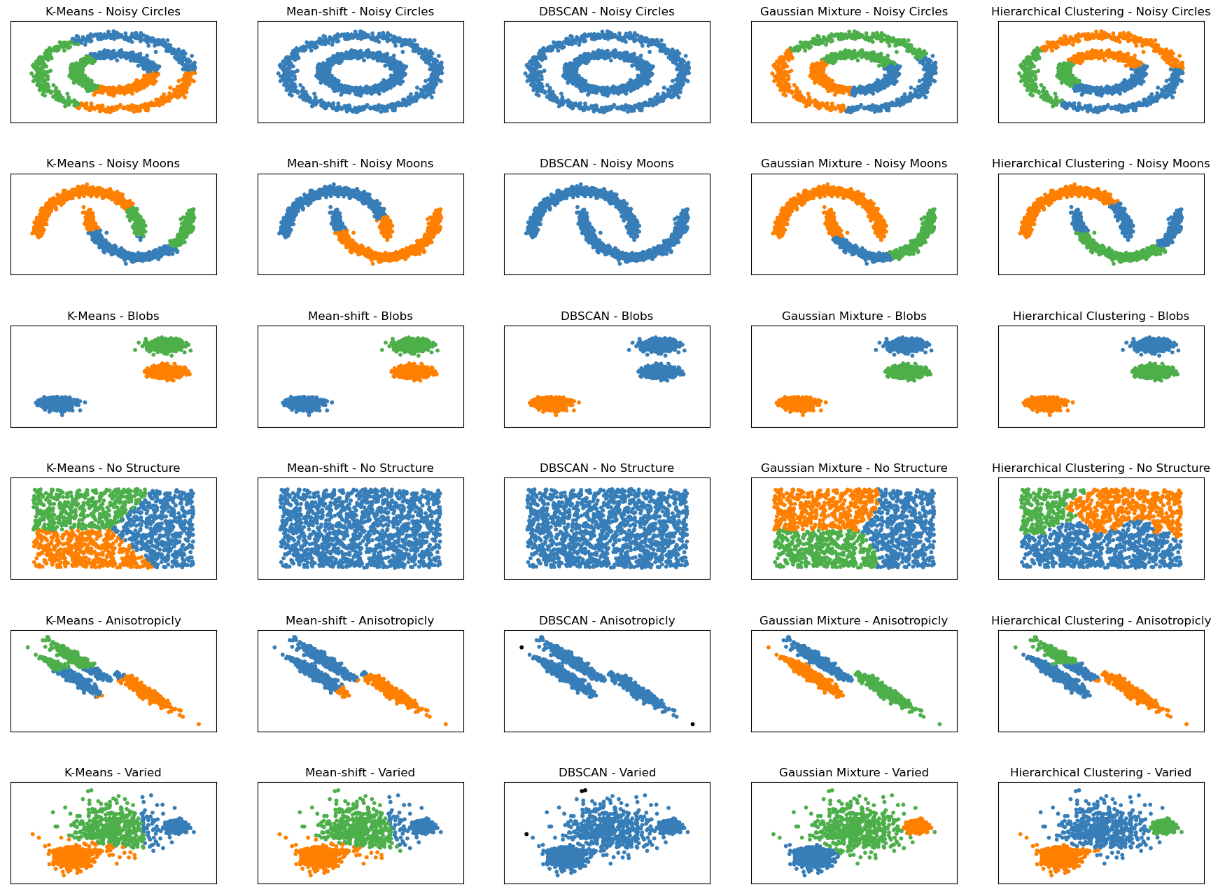
Clustering Algorithms - Image by Author
In the scikit-learn documentation, you will find similar graphs which inspired the image above. I limited it to the five most famous clustering algorithms and added the dataset's structure along the algorithm name, e.g., K-Means - Noisy Moons or K-Means Varied.
There are six different datasets shown, all generated by using scikit-learn:
- Noisy Circles: This dataset consists of a large circle containing a smaller circle that is not perfectly centered. The data also has random Gaussian noise added to it.
- Noisy Moons: This dataset consists of two interleaving half-moon shapes that are not linearly separable. The data also has random Gaussian noise added to it.
- Blobs: This dataset consists of randomly generated blobs that are relatively uniform in size and shape. The dataset contains three blobs.
- No Structure: This dataset consists of randomly generated data points with no inherent structure or clustering pattern.
- Anisotropicly Distributed: This dataset consists of randomly generated data points that are anisotropically distributed. The data points are generated with a specific transformation matrix to make them elongated along certain axes.
- Varied: This dataset consists of randomly generated blobs with varied variances. The dataset contains three blobs, each with a different standard deviation.
Seeing the plots and how each algorithm works on them will help us compare how well our algorithms perform on each dataset. This may help you in your data project if your data have the same structure as in these graphs.
Now let’s dig deeper into these five algorithms, starting with the K-Means algorithm.
K-Means
K-Means 2D | Image by Author
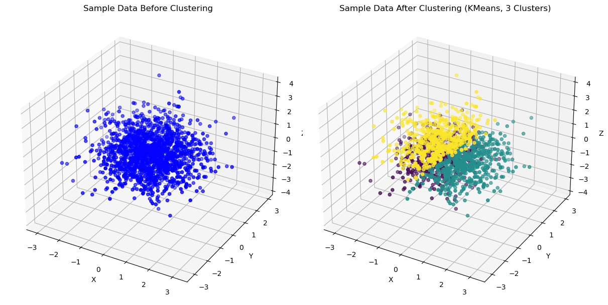
K Means 3D | Image by Author
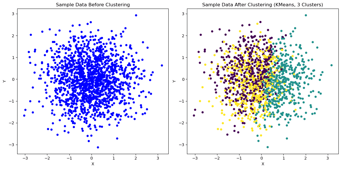
K-Means is a popular clustering algorithm that partitions a dataset into K distinct clusters, where K is a hyperparameter specified by the user.
The algorithm works by assigning each data point to the nearest cluster centroid and then recalculating the centroid based on the average of all the data points in that cluster.
This process continues until the centroids no longer move or a specified maximum number of iterations is reached.
It has also been used in various real-life applications, such as customer segmentation in e-commerce, disease clustering in healthcare, and image compression in computer vision.
To see the real-life applications of K-Means or other algorithms, continue reading. We will get to it in the later sections.
DBScan
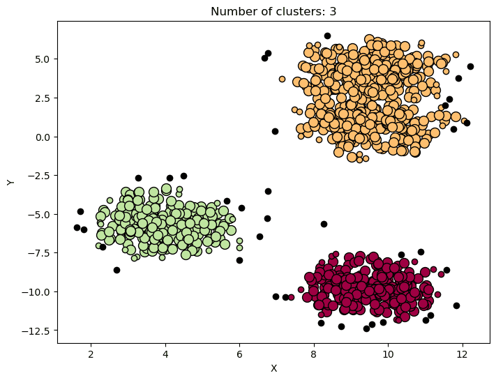
DBScan | Image by Author
DBScan (Density-Based Spatial Clustering of Applications with Noise) is a density-based clustering algorithm that identifies clusters as high-density regions separated by low-density regions.
The algorithm groups together point that are close to each other based on a density threshold and a minimum number of points.
DBScan is often used in outlier detection, spatial clustering, and image segmentation, where the goal is to identify distinct clusters in the data while also handling noisy or outlier data points.
Hierarchical Clustering
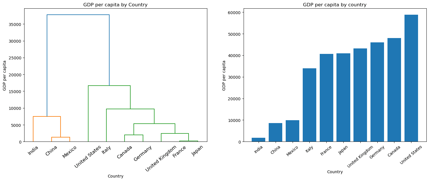
Hierarchical Clustering | Image by Author
Hierarchical Clustering is a clustering algorithm that builds a tree-like structure of clusters by merging or splitting clusters.
Depending on the approach taken, the algorithm can be agglomerative (bottom-up) or divisive (like the graph above).
Hierarchical Clustering has been used in various real-life applications such as social network analysis, image segmentation, and ecological research, where the goal is to identify meaningful relationships between clusters and subclusters.
Mean-Shift Clustering
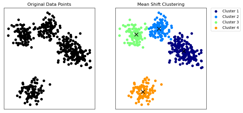
Mean-Shift Clustering | Image by Author
Mean-shift clustering is a non-parametric algorithm that doesn't require prior assumptions about the shape or number of clusters.
The algorithm works by shifting each data point towards the local mean (x in the above graph) until convergence, where the kernel density function estimates the local mean.
The mean-shift algorithm identifies clusters as high-density regions in the feature space.
Mean-shift clustering has been used in real-life applications such as image segmentation, object tracking in video surveillance, and anomaly detection in network intrusion detection, where the goal is to identify distinct regions or patterns in the data.
Gaussian Mixture Clustering
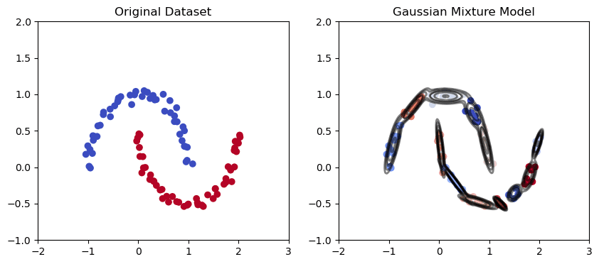
Gaussian Mixture Model in the moon-shaped data set | Image by Author
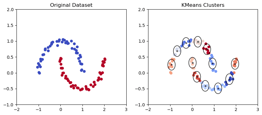
K Means Clustering Model in the moon-shaped data set | Image by Author
Gaussian Mixture is a probabilistic clustering algorithm that models the distribution of data points using a mixture of Gaussian distributions. The algorithm fits a set of Gaussian distributions to the data, where each Gaussian corresponds to a separate cluster.
Gaussian Mixture has been used in various real-life applications such as speech recognition, gene expression analysis, and face recognition, where the goal is to model the underlying distribution of the data and identify clusters based on the fitted Gaussian distributions.
As we can see from the graph above, the Gaussian mixture has a better capability of capturing trends in elliptical data points as above and drawing elliptical clusters.
Overall, each clustering algorithm has its unique strengths and weaknesses. The choice of algorithm depends on the problem at hand and the dataset's characteristics.
Understanding the nuances of each algorithm and its use cases is crucial for achieving accurate and meaningful results.
Clustering Evaluation Metrics
After applying the algorithm, you need to evaluate its performance to see whether there is room for improvement or change the algorithm if the performance of your algorithm does not meet the criteria. To do that, you should use evaluation metrics.
Here’s an overview of the most popular ones.
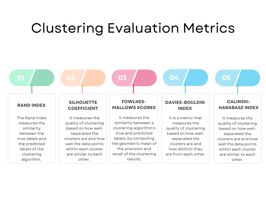
Image by Author
These are not all, of course. You can get the complete list on scikit-learn. It lists the following evaluation metrics: Rand Index, Mutual Information based scores, Silhouette Coefficient, Fowlkes-Mallows scores, Homogeneity, Completeness, V-measure, Calinski-Harabasz Index, Davies-Bouldin Index, Contingency Matrix, Pair Confusion Matrix.
Here you can see the official documents.
We will stick with the popular ones and start with the Rand Index.
Rand Index
The Rand Index evaluates the similarity between the true cluster labels and the predicted cluster labels.
The index ranges from 0 to 1, with 1 indicating a perfect match between the true and predicted labels.
The Rand Index is often used in image segmentation, text clustering, and document clustering, where the true labels of the data are known.
Silhouette Coefficient
The Silhouette Coefficient measures the quality of clustering based on how well-separated the clusters are and how similar are the data points within each cluster.
The coefficient ranges from -1 to 1, with 1 indicating a well-separated and compact cluster and -1 indicating an incorrect clustering.
The Silhouette Coefficient is often used in market segmentation, customer profiling, and product recommendation, where the goal is to identify meaningful clusters based on customer behavior and preferences.
Fowlkes-Mallows scores
The Fowlkes-Mallows index is named after two researchers, Edward Fowlkes and S.G. Mallows, who proposed the metric in 1983.
The index measures the similarity between a clustering algorithm's true and predicted labels.
The score ranges from 0 to 1, with 1 indicating a perfect match between the true and predicted labels.
The Fowlkes-Mallows score is often used in image segmentation, text clustering, and document clustering, where the true labels of the data are known.
Davies-Bouldin Index
The Davies-Bouldin Index is named after two researchers, David L. Davies and Donald W. Bouldin, who proposed the metric in 1979.
The index ranges from 0 to infinity, with lower values indicating better clustering quality.
It is handy for identifying the optimal number of clusters in the data and for detecting cases where the clusters overlap or are too similar to each other. However, the index assumes that the clusters are spherical and have similar densities, which may not always hold in real-world datasets.
The Davies-Bouldin Index is often used in market segmentation, customer profiling, and product recommendation, where the goal is to identify meaningful clusters based on customer behavior and preferences.
Calinski-Harabasz Index
The Calinski-Harabasz Index is named after T. Calinski and J. Harabasz, who proposed the metric in 1974.
The Calinski-Harabasz Index measures the quality of clustering based on how well-separated the clusters are and how well the data points within each cluster are similar to each other.
The index ranges from 0 to infinity, with higher values indicating better clustering.
The Calinski-Harabasz Index is often used in market segmentation, customer profiling, and product recommendation, where the goal is to identify meaningful clusters based on customer behavior and preferences.
Comparing Evaluation Metrics
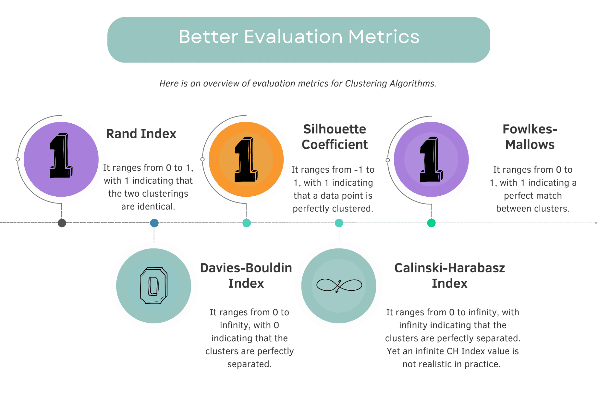
Image by Author
For the Rand Index, Silhouette Coefficient, and Fowlkes-Mallows scores, higher values indicate better clustering performance.
The best score is 1.
For Davies-Bouldin Index, lower values indicate better clustering performance.
The best score is 0.
For Calinski-Harabasz Index, the highest scores indicate better performance.
The best score is ∞. (infinity.)
In theory, the best score for the Calinski-Harabasz (CH) Index would be infinity, as it would indicate an extremely high between-cluster dispersion compared to the within-cluster dispersion. However, achieving an infinite CH Index value is not realistic in practice.
There is no fixed upper bound for the best score, as it depends on the specific data and clustering.
Don’t forget: there is no algorithm or script which is perfect. If you achieve the best scores with any of these evaluation metrics, it’s quite likely your model is overfitting.
How to Develop Multiple Clustering Algorithms at Once With scikit-learn?
The purpose here is to apply multiple clustering algorithms to the Iris dataset and calculate their performance using different evaluation metrics.
Here we will use the IRIS dataset.
You can find this dataset here.
The iris dataset is a famous multi-class classification dataset that contains 150 samples of iris flowers, each having four features (length and width of sepals and petals).
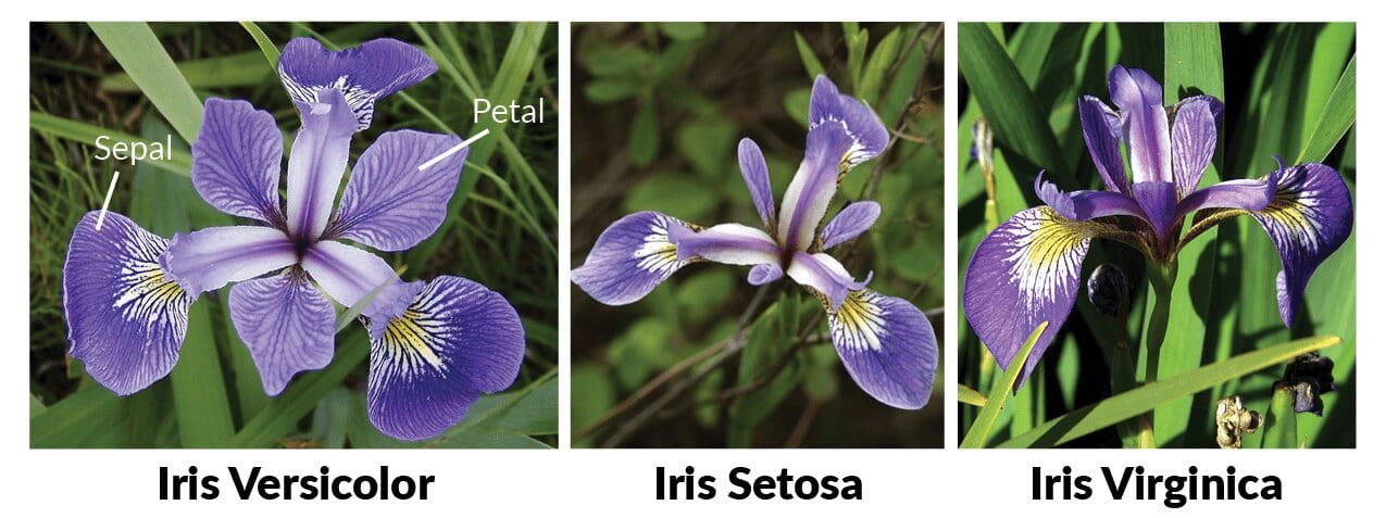
Image from Machine Learning in R for beginners
There are three classes in the dataset representing three types of iris flowers.
The dataset is commonly used for machine learning and pattern recognition tasks, particularly for testing and comparing different classification algorithms. It was introduced by British statistician and biologist Ronald Fisher in 1936.
Here we will write the code, which imports the necessary libraries to load the dataset, implements five clustering algorithms (DBSCAN, K-Means, Hierarchical Clustering, Gaussian Mixture Model, and Mean Shift), and evaluates their performance using five metrics.
To do that, we will add the evaluation metrics and algorithms in the dictionaries and apply them with two for loops each other.
But we have an exception here. The rand_score and fowlkes_mallows_score functions compare clustering results with true labels, so we will add the if-else block to provide that.
Then we will add these results to the data frame to do further analysis.
Here is the code.
import numpy as np
import pandas as pd
import matplotlib.pyplot as plt
from sklearn.datasets import load_iris
from sklearn.cluster import (
    DBSCAN,
    KMeans,
    AgglomerativeClustering,
    MeanShift,
)
from sklearn.mixture import GaussianMixture
from sklearn.metrics import (
    silhouette_score,
    calinski_harabasz_score,
    davies_bouldin_score,
    rand_score,
    fowlkes_mallows_score,
)

# Load the Iris dataset
iris = load_iris()
X = iris.data
y = iris.target

# Implement clustering algorithms
dbscan = DBSCAN(eps=0.5, min_samples=5)
kmeans = KMeans(n_clusters=3, random_state=42)
agglo = AgglomerativeClustering(n_clusters=3)
gmm = GaussianMixture(n_components=3, covariance_type="full")
ms = MeanShift()

# Evaluate clustering algorithms with three evaluation metrics
labels = {
    "DBSCAN": dbscan.fit_predict(X),
    "K-Means": kmeans.fit_predict(X),
    "Hierarchical": agglo.fit_predict(X),
    "Gaussian Mixture": gmm.fit_predict(X),
    "Mean Shift": ms.fit_predict(X),
}

metrics = {
    "Silhouette Score": silhouette_score,
    "Calinski Harabasz Score": calinski_harabasz_score,
    "Davies Bouldin Score": davies_bouldin_score,
    "Rand Score": rand_score,
    "Fowlkes-Mallows Score": fowlkes_mallows_score,
}


for name, label in labels.items():
    for metric_name, metric_func in metrics.items():
        if metric_name in ["Rand Score", "Fowlkes-Mallows Score"]:
            score = metric_func(y, label)
        else:
            score = metric_func(X, label)
        pred_df = pred_df.append(
            {"Algorithm": name, "Metric": metric_name, "Score": score},
            ignore_index=True,
        )
# Display the DataFrame
pred_df.head(10)
Here is the output.
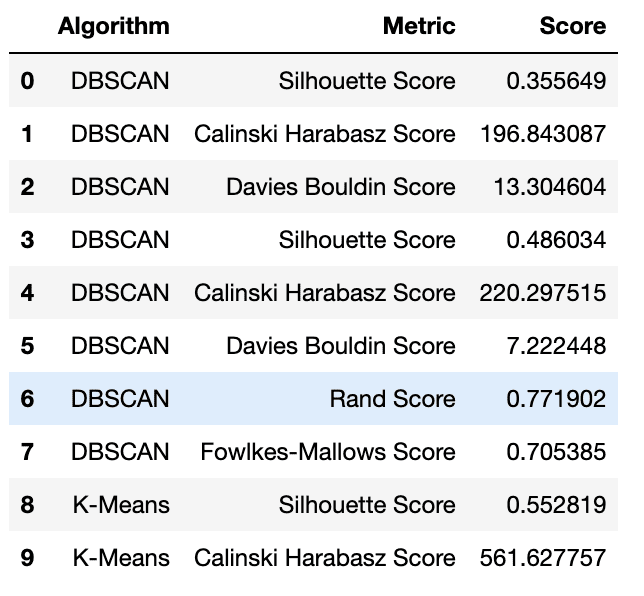
Prediction DataFrame | Image by Author
Now, let’s make a visualization to see the result better. Here the aim is to create visuals of the clustering algorithm's evaluation metrics.
The following code pivots the data to have algorithms as columns and metrics as rows and then generates bar charts for each metric. This allows for easy comparison of the clustering algorithms' performance across different evaluation measures.
Here is the code.
import pandas as pd
import numpy as np
import matplotlib.pyplot as plt

# Pivot the data to have algorithms as columns and metrics as rows
pivoted_df = pred_df.pivot(
    index="Metric", columns="Algorithm", values="Score"
)

# Define the three metrics to plot
metrics = [
    "Silhouette Score",
    "Calinski Harabasz Score",
    "Davies Bouldin Score",
]

# Define a colormap to use for each algorithm
cmap = plt.get_cmap("Set3")

# Plot a bar chart for each metric
fig, axs = plt.subplots(nrows=1, ncols=3, figsize=(15, 5))

# Add a main title to the figure
fig.suptitle("Comparing Evaluation Metrics", fontsize=16, fontweight="bold")

for i, metric in enumerate(metrics):
    ax = pivoted_df.loc[metric].plot(kind="bar", ax=axs[i], rot=45)
    ax.set_xticklabels(ax.get_xticklabels(), ha="right")
    ax.set_ylabel(metric)
    ax.set_title(metric, fontstyle="italic")

    # Iterate through the algorithm names and set the color for each bar
    for j, alg in enumerate(pivoted_df.columns):
        ax.get_children()[j].set_color(cmap(j))
plt.show()
Here is the output.
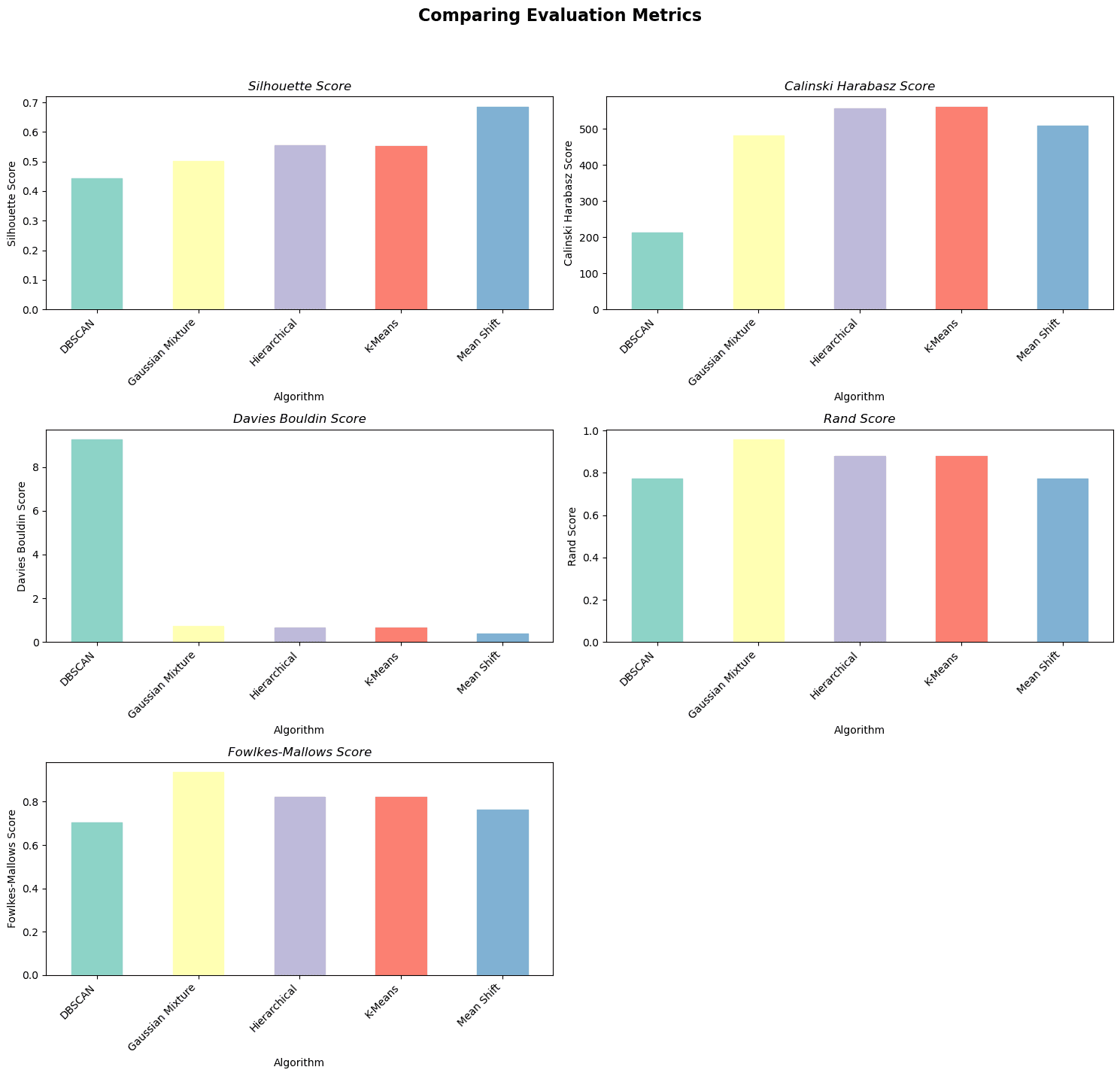
Image by Author
In summary, the Mean Shift algorithm performs the best according to the Silhouette Score and Davies Bouldin Score.
The K-Means algorithm performs the best according to the Calinski Harabasz Score, and GMM performs the best according to the Rand Score and Fowlkes-Mallows Score.
There is no clear winner among the clustering algorithms, as each one performs well on different metrics.
The choice of the best algorithm depends on the specific requirements and the importance assigned to each evaluation metric in your clustering problem.
Clustering Real-Life Applications
Now, let’s see the real-life examples of both our algorithms and evaluation metrics to grasp the logic even further.
Here’s the overview of the examples we’ll talk about in detail.
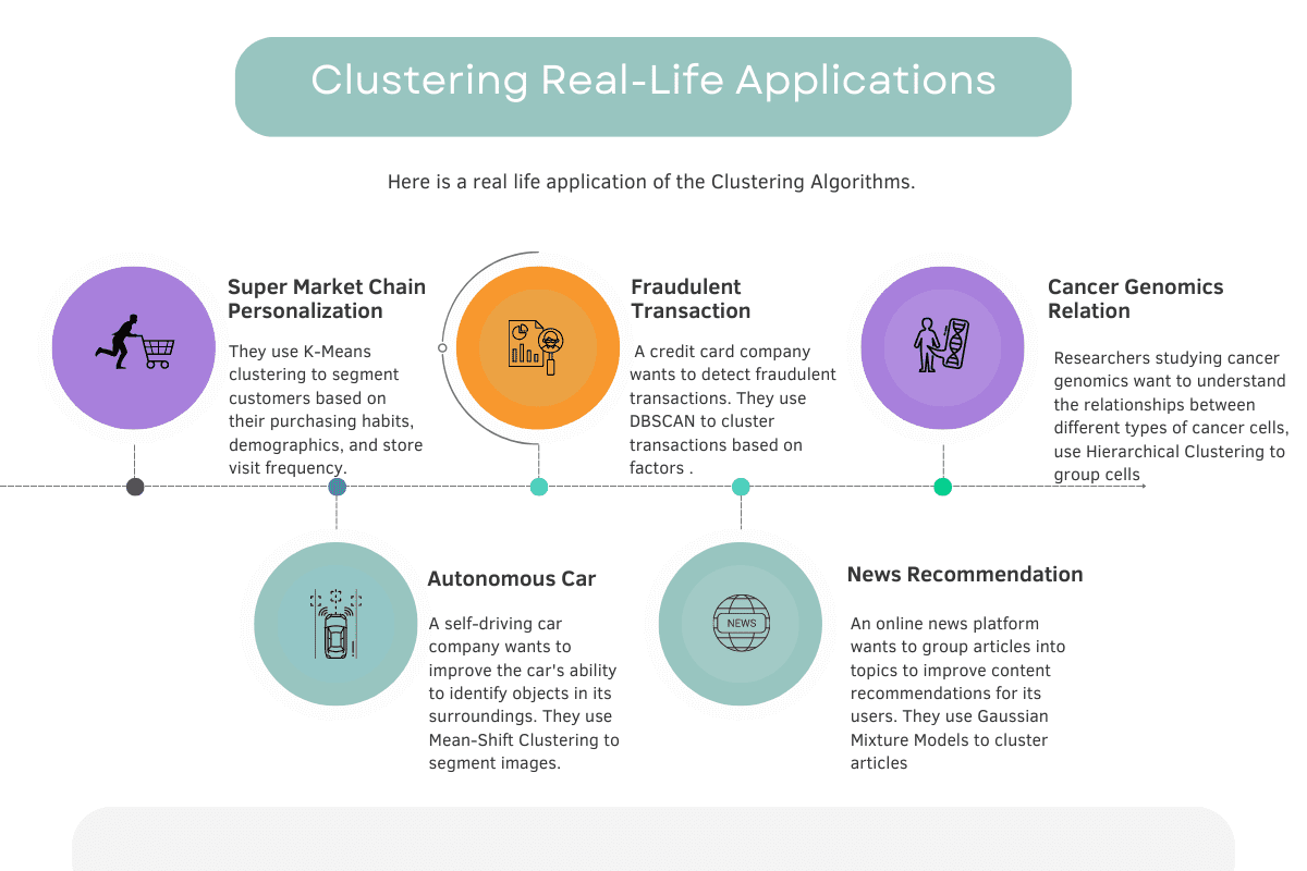
Image by Author
Super Market Chain Personalization
Image by Author
Real-life example: A supermarket chain wants to create personalized marketing campaigns for its customers. They use K-Means clustering to segment customers based on their purchasing habits, demographics, and store visit frequency. These segments help the company tailor its marketing messages to engage better and serve its customers.
Algorithm: K-Means clustering
K-Means is chosen because it is a simple, efficient, and widely-used clustering algorithm that works well with large datasets. It can quickly identify patterns and create distinct customer segments based on the input features.
Evaluation metrics: Silhouette Score
The Silhouette Score is used to evaluate the quality of customer segmentation by measuring how well each data point fits within its assigned cluster compared to other clusters. This helps ensure the clusters are compact and well-separated, which is essential for creating effective personalized marketing campaigns.
Fraudulent Transaction
Image by Author
Real-life example: A credit card company wants to detect fraudulent transactions. They use DBSCAN to cluster transactions based on factors like transaction amount, time, and location. Unusual transactions that don't fit into any cluster are flagged as potential frauds for further investigation.
Algorithm: DBSCAN
DBSCAN is chosen because it is a density-based clustering algorithm that can identify clusters of varying shapes and sizes, as well as detect noise points that do not belong to any cluster. This makes it suitable for detecting unusual patterns or outliers, such as potentially fraudulent transactions.
Evaluation metrics: Silhouette Score
The Silhouette Score is chosen as an evaluation metric in this case because it helps assess the effectiveness of DBSCAN by separating normal transactions from potential outliers representing fraud.
A higher Silhouette Score indicates that the clusters of regular transactions are well separated from each other and the noise points (outliers). This separation makes it easier to identify and flag suspicious transactions that deviate significantly from normal patterns.
Cancer Genomics Relation
Image by Author
Real-life example: Researchers studying cancer genomics want to understand the relationships between different types of cancer cells. They use Hierarchical Clustering to group cells based on their gene expression patterns. The resulting clusters help them identify commonalities and differences between cancer types and develop targeted therapies.
Algorithm: Agglomerative Hierarchical Clustering
Agglomerative Hierarchical Clustering is chosen because it creates a tree-like structure (dendrogram) that allows researchers to visualize and interpret the relationships between cancer cells at multiple levels of granularity. This approach can reveal nested subgroups of cells and helps researchers understand the hierarchical organization of cancer types based on their gene expression patterns.
Evaluation metrics: Calinski-Harabasz Index
The Calinski-Harabasz Index is chosen in this case because it measures the ratio of between-cluster dispersion to within-cluster dispersion. For cancer genomics, it helps researchers evaluate the clustering quality in terms of how distinct and well-separated the groups of cancer cells are based on their gene expression patterns.
Autonomous Car
Image by Author
Real-life example: A self-driving car company wants to improve the car's ability to identify objects in its surroundings. They use Mean-Shift Clustering to segment images captured by the car's cameras into different regions based on color and texture, which helps the car recognize and track objects like pedestrians and other vehicles.
Algorithm: Mean Shift Clustering
Mean Shift clustering is chosen because it is a non-parametric, density-based algorithm that can automatically adapt to the underlying structure and scale of the data.
This makes it particularly suitable for image segmentation tasks, where the number of clusters or regions may not be known in advance, and the shapes of the regions can be complex and irregular.
Evaluation metrics: Fowlkes-Mallows Score (FMS)
The Fowlkes-Mallows Score is chosen in this case because it measures the similarity between two clusterings, typically comparing the algorithm's output to a ground-truth clustering.
In the context of self-driving cars, the FMS can be used to assess how well the Mean Shift clustering algorithm segments the images compared to human-labeled segmentations.
News Recommendation
Image by Author
Real-life example: An online news platform wants to group articles into topics to improve content recommendations for its users. They use Gaussian Mixture Models to cluster articles based on features extracted from their texts, such as word frequency and term co-occurrence. By identifying distinct topics, the platform can recommend articles more relevant to a user's interests.
Algorithm: Gaussian Mixture Model (GMM) clustering
Gaussian Mixture Models are chosen because they are a probabilistic, generative approach that can model complex, overlapping clusters. This is particularly useful for text data, where articles may belong to multiple topics or have shared features. GMM can capture these nuances and provide a soft clustering, assigning each article a probability of belonging to each topic.
Evaluation metrics: Silhouette Coefficient
The Silhouette Coefficient is chosen because it measures the compactness and separation of the clusters, helping assess the quality of the topic assignments.
A higher Silhouette Coefficient indicates that the articles within a topic are more similar to each other and distinct from other topics, which is important for accurate content recommendations.
If you want to know more about Unsupervised algorithms, here you can collect more information on “Unsupervised Learning Algorithms”. Also, check out “Supervised vs Unsupervised Learning” the two approaches that we should know in the world of machine learning.
Conclusion
In conclusion, clustering is an essential unsupervised learning technique used to find similarities or patterns in data without prior knowledge of class labels.
We discussed different clustering algorithms, including K-Means, Mean Shift, DBScan, Gaussian Mixture, and Hierarchical Clustering, along with their use cases and real-life applications.
Additionally, we explored various evaluation metrics, including the Silhouette Coefficient, Calinski-Harabasz Index, and Davies-Bouldin Index, which help us assess the quality of clustering results.
We also learned how to develop multiple clustering algorithms simultaneously using scikit-learn and evaluated them using the metrics we had already discovered.
Finally, we discussed some popular applications that utilized clustering algorithms to solve real-world problems.
If you still have questions, here is an article explaining Clustering and its algorithms.
Clustering has a wide range of applications, from customer segmentation in marketing to image recognition in computer vision, and it is an essential tool for discovering hidden patterns and insights in data.
Nate Rosidi is a data scientist and in product strategy. He's also an adjunct professor teaching analytics, and is the founder of StrataScratch, a platform helping data scientists prepare for their interviews with real interview questions from top companies. Connect with him on Twitter: StrataScratch or LinkedIn.