Advanced Feature Selection Techniques for Machine Learning Models
Mastering Feature Selection: An Exploration of Advanced Techniques for Supervised and Unsupervised Machine Learning Models.

Image by Author
Machine learning is undeniably the shining star of the new era. It forms the backbone of various major technologies that have become integral to our daily lives, such as facial recognition (supported by Convolutional Neural Networks or CNN), speech recognition (leveraging CNN and Recurrent Neural Networks or RNN), and the increasingly popular chatbots like ChatGPT (powered by Reinforcement Learning from Human Feedback, RLHF).
Numerous methods are available today to enhance the performance of a machine learning model. These methods can give your project a competitive edge by delivering superior performance.
In this discussion, we'll delve into the realm of feature selection techniques. But before we proceed, let's clarify: what exactly is feature selection?
What Is the Feature Selection?
Feature selection is the process of choosing the best features for your model. This process might differ from one technique to another, but the main goal is to find out which features have more impact on your model.
Why Should We Do Feature Selection?
Because sometimes, having too many features might harm your machine learning model. How?
There might be too many different reasons. For example, these features might be related to each other, which can cause multicollinearity, ruining your model’s performance.
Another potential issue is related to computational power. The presence of too many features necessitates more computational power to execute the task concurrently, which could require more resources and, consequently, increased costs.
Certainly, there may be other reasons as well. But these examples should give you a general idea of the potential problems. However, there's one more important aspect to understand before we delve further into this topic.
Which Feature Selection Method Will Be Better for My Model?
Yes, that is a great question and should be answered before beginning the project. But it’s not easy to give a generic answer.
The choice of feature selection model relies on the type of data you have and the aim of your project.
For example, filter-based methods such as the chi-squared test or mutual information gain are typically used for feature selection in categorical data. The wrapper-based methods like forward or backward selection are suitable for numerical data.
Yet, it's good to know that many feature selection methods can handle both categorical and numerical data.
For example, lasso regression, decision trees, and random forest can handle both types of data quite well.
In terms of supervised and unsupervised feature selection, supervised methods like recursive feature elimination or decision trees are good for labeled data. Unsupervised methods like principal component analysis (PCA) or independent component analysis (ICA) are used for unlabeled data.
Ultimately, the choice of feature selection method should be based on the specific characteristics of your data and the goals of your project.
Take a look at the overview of the topics we’ll discuss in the article. Make yourself familiar with it, and let’s start with the supervised feature selection techniques.
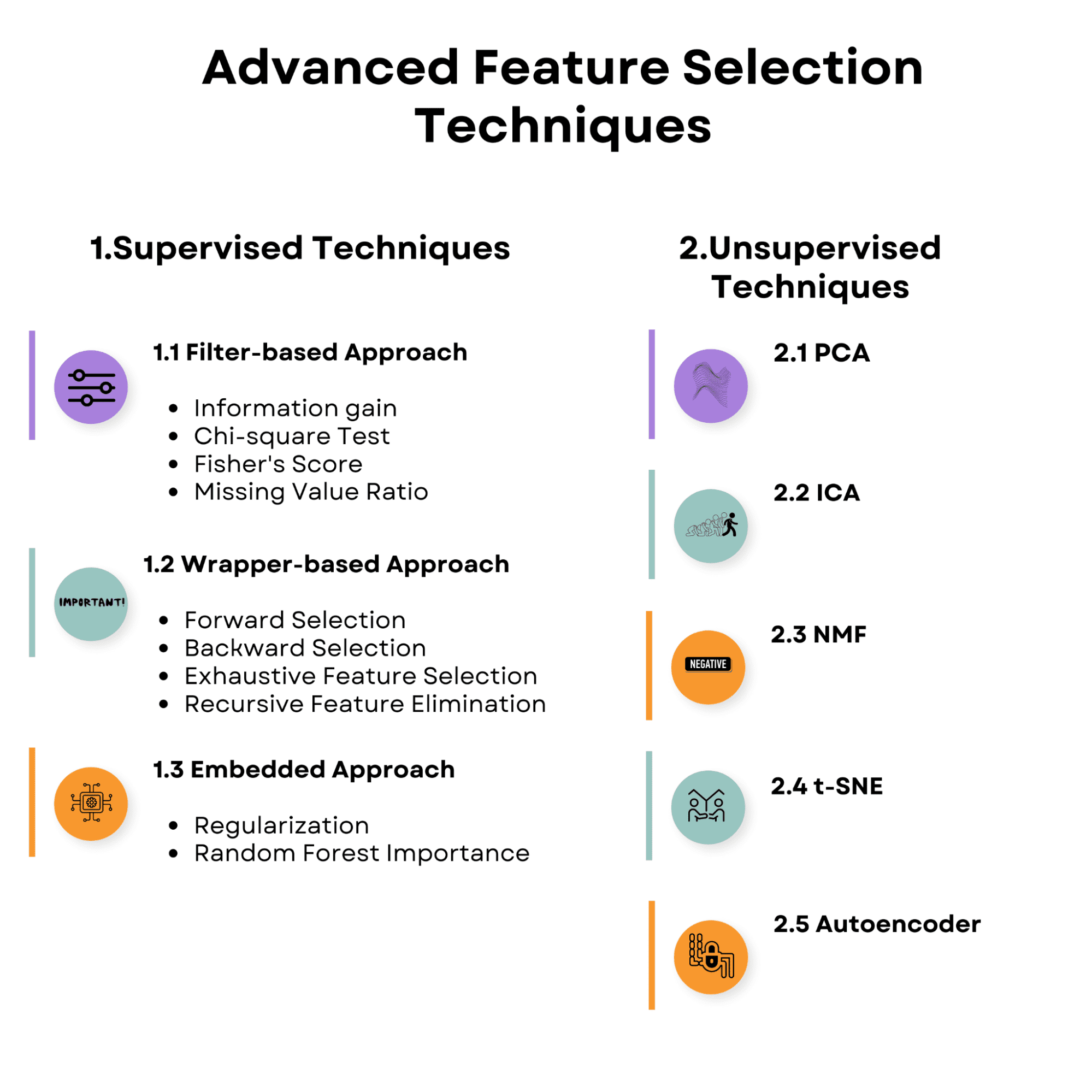
Image by Author
1. Supervised Feature Selection Techniques
Feature selection strategies in supervised learning aim to discover the most relevant features for predicting the target variable by using the relationship between the input features and the target variable. These strategies might help improve model performance, reduce overfitting, and lower the computational cost of training the model.
Here’s the overview of the supervised feature selection techniques we’ll talk about.
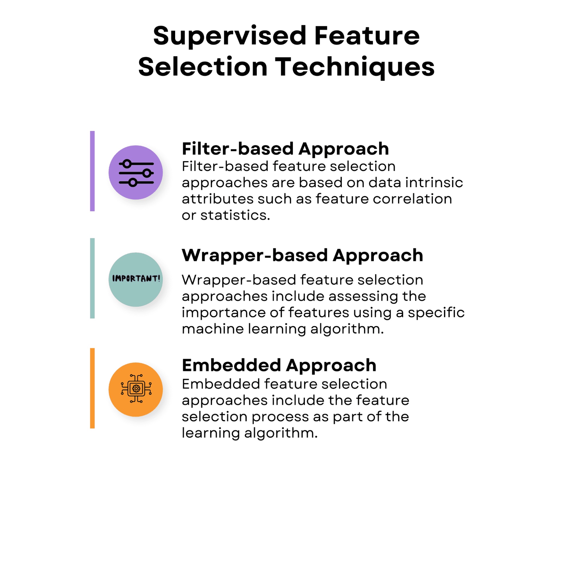
Image by Author
1.1 Filter-Based Approach
Filter-based feature selection approaches are based on data intrinsic attributes such as feature correlation or statistics. These approaches assess the value of each characteristic alone or in pairs without taking into account the performance of a particular learning algorithm.
Filter-based approaches are computationally efficient and may be used with a variety of learning algorithms. However, because they do not account for the interaction between the features and the learning method, they may not always capture the ideal feature subset for a certain algorithm.
Take a look at the overview of the filter-based approaches, and then we’ll discuss each.
Image by Author
Information Gain
Information Gain is a statistic that measures the reduction in entropy (uncertainty) for a specific feature by dividing the data according to that characteristic. It is often used in decision tree algorithms and also has useful features. The higher a feature's information gain, the more useful it is for decision-making.
Now, let’s apply information gain by using a prebuilt diabetes dataset.
The diabetes dataset contains physiological features related to predicting the progression of diabetes.
- age: Age in years
- sex: Gender (1 = male, 0 = female)
- BMI: Body mass index, calculated as weight in kilograms divided by the square of height in meters
- bp: Average blood pressure (mm Hg)
- s1, s2, s3, s4, s5, s6: Blood serum measurements of six different blood chemicals (including glucose),
The following code demonstrates how to apply the Information Gain method. This code uses the diabetes dataset from the sklearn library as an example.
import numpy as np
import matplotlib.pyplot as plt
from sklearn.datasets import load_diabetes
from sklearn.feature_selection import mutual_info_regression

# Load the diabetes dataset
data = load_diabetes()

# Split the dataset into features and target
X = data.data
y = data.target
The primary objective of this code is to calculate feature importance scores based on Information Gain, which helps identify the most relevant features for the predictive model. By determining these scores, you can make informed decisions about which features to include or exclude from your analysis, ultimately leading to improved model performance, reduced overfitting, and faster training times.
To achieve this, this code calculates Information Gain scores for each feature in the dataset and stores them in a dictionary.
import numpy as np
import matplotlib.pyplot as plt
from sklearn.datasets import load_diabetes
from sklearn.feature_selection import mutual_info_regression

# Load the diabetes dataset
data = load_diabetes()

# Split the dataset into features and target
X = data.data
y = data.target

# Apply Information Gain
ig = mutual_info_regression(X, y)

# Create a dictionary of feature importance scores
feature_scores = {}
for i in range(len(data.feature_names)):
    feature_scores[data.feature_names[i]] = ig[i]
The features are then sorted in descending order according to their scores.
# Sort the features by importance score in descending order
sorted_features = sorted(feature_scores.items(), key=lambda x: x[1], reverse=True)

# Print the feature importance scores and the sorted features
for feature, score in sorted_features:
    print('Feature:', feature, 'Score:', score)
We will visualize the sorted feature importance scores as a horizontal bar chart, allowing you to easily compare the relevance of different features for the given task.
This visualization is particularly helpful when deciding which features to retain or discard while building a machine-learning model.
# Plot a horizontal bar chart of the feature importance scores
fig, ax = plt.subplots()
y_pos = np.arange(len(sorted_features))
ax.barh(y_pos, [score for feature, score in sorted_features], align="center")
ax.set_yticks(y_pos)
ax.set_yticklabels([feature for feature, score in sorted_features])
ax.invert_yaxis()  # Labels read top-to-bottom
ax.set_xlabel("Importance Score")
ax.set_title("Feature Importance Scores (Information Gain)")

# Add importance scores as labels on the horizontal bar chart
for i, v in enumerate([score for feature, score in sorted_features]):
    ax.text(v + 0.01, i, str(round(v, 3)), color="black", fontweight="bold")
plt.show()
Let’s see the whole code.
import numpy as np
import matplotlib.pyplot as plt
from sklearn.datasets import load_diabetes
from sklearn.feature_selection import mutual_info_regression

# Load the diabetes dataset
data = load_diabetes()

# Split the dataset into features and target
X = data.data
y = data.target

# Apply Information Gain
ig = mutual_info_regression(X, y)

# Create a dictionary of feature importance scores
feature_scores = {}
for i in range(len(data.feature_names)):
    feature_scores[data.feature_names[i]] = ig[i]
# Sort the features by importance score in descending order
sorted_features = sorted(feature_scores.items(), key=lambda x: x[1], reverse=True)

# Print the feature importance scores and the sorted features
for feature, score in sorted_features:
    print("Feature:", feature, "Score:", score)
# Plot a horizontal bar chart of the feature importance scores
fig, ax = plt.subplots()
y_pos = np.arange(len(sorted_features))
ax.barh(y_pos, [score for feature, score in sorted_features], align="center")
ax.set_yticks(y_pos)
ax.set_yticklabels([feature for feature, score in sorted_features])
ax.invert_yaxis()  # Labels read top-to-bottom
ax.set_xlabel("Importance Score")
ax.set_title("Feature Importance Scores (Information Gain)")

# Add importance scores as labels on the horizontal bar chart
for i, v in enumerate([score for feature, score in sorted_features]):
    ax.text(v + 0.01, i, str(round(v, 3)), color="black", fontweight="bold")
plt.show()
Here is the output.
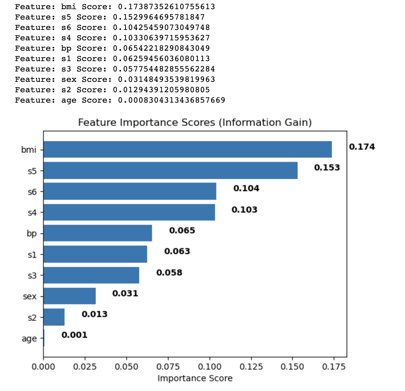
The output shows the feature importance scores calculated using the Information Gain method for each feature in the diabetes dataset. The features are sorted in descending order based on their scores, which indicate their relative importance in predicting the target variable.
The results are as follows:
- Body mass index (bmi) has the highest importance score (0.174), indicating that it has the most significant influence on the target variable in the diabetes dataset.
- Serum measurement 5 (s5) follows with a score of 0.153, making it the second most important feature.
- Serum measurement 6 (s6), serum measurement 4 (s4), and blood pressure (bp) have moderate importance scores, ranging from 0.104 to 0.065.
- The remaining features, such as serum measurements 1, 2, and 3 (s1, s2, s3), sex, and age, have relatively lower importance scores, indicating that they contribute less to the predictive power of the model.
By analyzing these feature importance scores, you can decide which features to include or exclude from your analysis to improve the performance of your machine learning model. In this case, you might consider retaining features with higher importance scores, such as bmi and s5, while potentially removing or further investigating features with lower scores, such as age and s2.
Chi-square Test
The Chi-square test is a statistical test used to assess the relationship between two categorical variables. It is used in feature selection to analyze the relationship between a categorical feature and the target variable. A greater Chi-square score shows a stronger link between the feature and the target, showing that the feature is more important for the classification job.
While the Chi-square test is a commonly used feature selection method, it is typically used for categorical data, where the features and target variables are discrete.
Fisher’s Score
Fisher's Discriminant Ratio, commonly known as Fisher's Score, is a feature selection approach that ranks features based on their ability to differentiate various classes in a dataset. It may be used for continuous features in a classification problem.
Fisher's Score is calculated as the ratio of between-class and within-class variance. A higher Fisher's Score implies the characteristic is more discriminative and valuable for classification.
To use Fisher's Score for feature selection, compute a score for each continuous feature and rank them according to their scores. The model considers features with a higher Fisher's Score more important.
Missing Value Ratio
The Missing Value Ratio is a straightforward feature selection method that makes decisions based on the number of missing values in a feature.
Features having a significant proportion of missing values may be uninformative and may harm the model's performance. You can filter out features with too many missing values by specifying a threshold for the acceptable missing value ratio.
To use the Missing Value Ratio for feature selection, follow these steps:
- Calculate the missing value ratio for each feature by dividing the number of missing values by the total number of instances in the dataset.
- Set a threshold for the acceptable missing value ratio (e.g., 0.8, meaning that a feature should have at most 80% of its values missing to be considered).
- Filter out features that have a missing value ratio above the threshold.
1.2 Wrapper-Based Approach
Wrapper-based feature selection approaches include assessing the importance of features using a specific machine learning algorithm. They seek the best subset of features by experimenting with various feature combinations and evaluating their performance with the selected method.
Because of the huge amount of available feature subsets, wrapper-based approaches can be computationally costly, especially when working with high-dimensional datasets.
However, they often outperform filter-based approaches because they consider the relationship between features and the learning algorithm.

Image by Author
Forward Selection
In forward selection, you start with an empty feature set and iteratively add features to the set. At each step, you evaluate the model's performance with the current feature set and the additional feature. The feature that results in the best performance improvement is added to the set.
The process continues until no significant improvement in performance is observed, or a predefined number of features is reached.
The following code demonstrates the application of forward selection, a wrapper-based supervised feature selection technique.
The example uses the breast cancer dataset from the sklearn library. The Breast Cancer dataset, also known as the Wisconsin Diagnostic Breast Cancer (WDBC) dataset, is a commonly used pre-built dataset for classification. And here, the main objective is building predictive models for diagnosing breast cancer as either malignant (cancerous) or benign (non-cancerous).
For the sake of our model, we will select a different number of features to see how performance changes accordingly, but first, let’s load the libraries, dataset, and variables.
import numpy as np
import pandas as pd
from sklearn.datasets import load_breast_cancer
from sklearn.linear_model import LogisticRegression
from sklearn.model_selection import train_test_split
from mlxtend.feature_selection import SequentialFeatureSelector as SFS

# Load the breast cancer dataset
data = load_breast_cancer()

# Split the dataset into features and target
X = data.data
y = data.target
The objective of the code is to identify an optimal subset of features for a logistic regression model using forward selection. This technique starts with an empty set of features and iteratively adds the features that improve the model's performance based on a specified evaluation metric. In this case, the metric used is accuracy.
The next part of the code employs the SequentialFeatureSelector from the mlxtend library to perform forward selection. It is configured with a logistic regression model, the desired number of features, and 5-fold cross-validation. The forward selection object is fitted to the training data, and the selected features are printed.
import numpy as np
import pandas as pd
from sklearn.datasets import load_breast_cancer
from sklearn.linear_model import LogisticRegression
from sklearn.model_selection import train_test_split
from mlxtend.feature_selection import SequentialFeatureSelector as SFS

# Load the breast cancer dataset
data = load_breast_cancer()

# Split the dataset into features and target
X = data.data
y = data.target

# Split the dataset into training and testing sets
X_train, X_test, y_train, y_test = train_test_split(X, y, test_size=0.3, random_state=0)

# Define the logistic regression model
model = LogisticRegression()

# Define the forward selection object
sfs = SFS(model,
          k_features=5,
          forward=True,
          floating=False,
          scoring='accuracy',
          cv=5)

# Perform forward selection on the training set
sfs.fit(X_train, y_train)
Additionally, we need to evaluate the performance of the selected features on the testing set and visualize the model's performance with different feature subsets in a line chart.
The chart will show the cross-validated accuracy as a function of the number of features, providing insights into the trade-off between model complexity and predictive performance.
By analyzing the output and the chart, you can determine the optimal number of features to include in your model, ultimately improving its performance and reducing overfitting.
# Print the selected features
print('Selected Features:', sfs.k_feature_names_)

# Evaluate the performance of the selected features on the testing set
accuracy = sfs.k_score_
print('Accuracy:', accuracy)

# Plot the performance of the model with different feature subsets
sfs_df = pd.DataFrame.from_dict(sfs.get_metric_dict()).T
sfs_df['avg_score'] = sfs_df['avg_score'].astype(float)
fig, ax = plt.subplots()
sfs_df.plot(kind='line', y='avg_score', ax=ax)
ax.set_xlabel('Number of Features')
ax.set_ylabel('Accuracy')
ax.set_title('Forward Selection Performance')
plt.show()
Here is the whole code.
import numpy as np
import pandas as pd
from sklearn.datasets import load_breast_cancer
from sklearn.linear_model import LogisticRegression
from sklearn.model_selection import train_test_split
from mlxtend.feature_selection import SequentialFeatureSelector as SFS

# Load the breast cancer dataset
data = load_breast_cancer()

# Split the dataset into features and target
X = data.data
y = data.target

# Split the dataset into training and testing sets
X_train, X_test, y_train, y_test = train_test_split(X, y, test_size=0.3, random_state=0)

# Define the logistic regression model
model = LogisticRegression()

# Define the forward selection object
sfs = SFS(model, k_features=5, forward=True, floating=False, scoring="accuracy", cv=5)

# Perform forward selection on the training set
sfs.fit(X_train, y_train)

# Print the selected features
print("Selected Features:", sfs.k_feature_names_)

# Evaluate the performance of the selected features on the testing set
accuracy = sfs.k_score_
print("Accuracy:", accuracy)

# Plot the performance of the model with different feature subsets
sfs_df = pd.DataFrame.from_dict(sfs.get_metric_dict()).T
sfs_df["avg_score"] = sfs_df["avg_score"].astype(float)
fig, ax = plt.subplots()
sfs_df.plot(kind="line", y="avg_score", ax=ax)
ax.set_xlabel("Number of Features")
ax.set_ylabel("Accuracy")
ax.set_title("Forward Selection Performance")
plt.show()
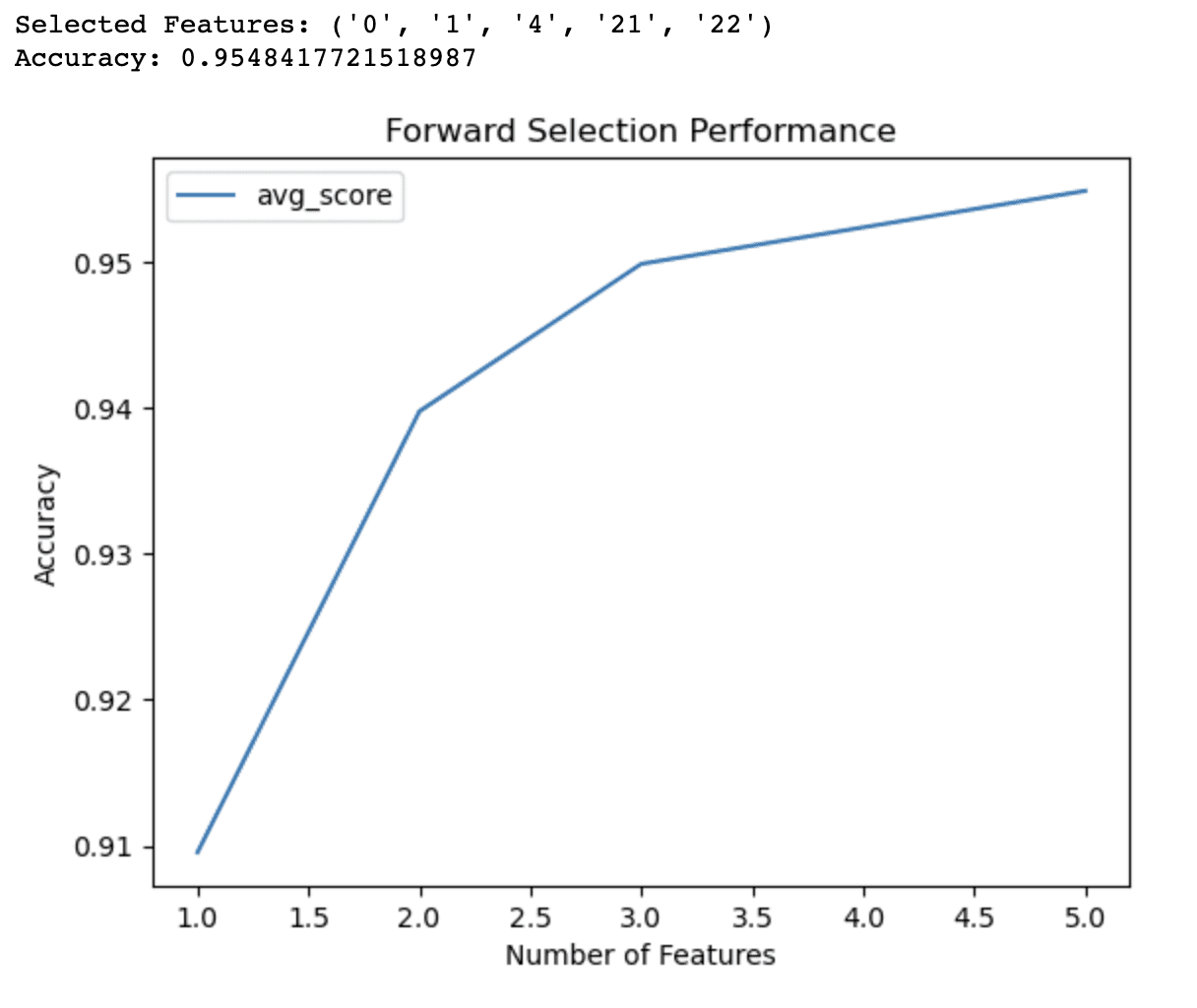
The output of the forward selection code demonstrates that the algorithm has identified a subset of 5 features that yield the best accuracy (0.9548) for the logistic regression model on the breast cancer dataset. These selected features are identified by their indices: 0, 1, 4, 21, and 22.
The line graph provides additional insights into the performance of the model with different numbers of features. It shows that:
- With just 1 feature, the model achieves an accuracy of around 91%.
- Adding a second feature increases the accuracy to 94%.
- With 3 features, the accuracy further improves to 95%.
- Including 4 features pushes the accuracy slightly above 95%.
Beyond 4 features, the improvements in accuracy become less significant. This information can help you make informed decisions about the trade-offs between model complexity and predictive performance. Based on these results, you might decide to use only 3 or 4 features in your model to balance accuracy and simplicity.
Backward Selection
The opposite of forward selection is backward selection. You begin with the entire feature set and gradually eliminate features from it.
At each phase, you measure the model's performance with the current feature set minus the feature to be deleted.
The feature that causes the least amount of performance reduction gets eliminated from the set.
The procedure is repeated until there is no substantial increase in performance or a preset number of features is reached.
Backward and forward selections are categorized as a sequential feature selection; you can learn more here.
Exhaustive Feature Selection
Exhaustive feature selection compares the performance of all possible feature subsets and chooses the best-performing subset. This approach is computationally demanding, especially for large datasets, yet it ensures the best feature subset.
Recursive Feature Elimination
Recursive feature elimination starts with the whole feature set and eliminates features repeatedly depending on their relevance as judged by the learning algorithm. The least important feature is removed at each step, and the model is retrained. The method is repeated until a predetermined number of features are achieved.
1.3 Embedded Approach
Embedded feature selection approaches include the feature selection process as part of the learning algorithm.
This implies that throughout the training phase, the learning algorithm not only optimizes the model parameters but also picks the most important characteristics. Embedded methods can be more effective than wrapper methods since they do not require an external feature selection procedure.
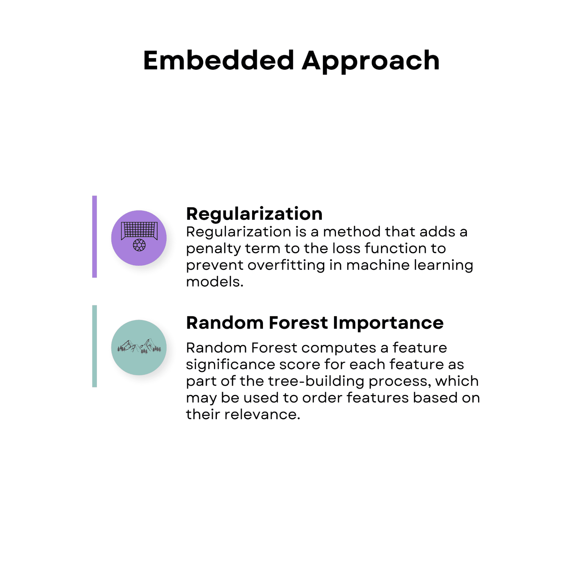
Image by Author
Regularization
Regularization is a method that adds a penalty term to the loss function to prevent overfitting in machine learning models.
Regularization methods, such as lasso (L1 regularization) and ridge (L2 regularization), can be used in conjunction with feature selection to decrease the coefficients of less significant features towards zero, thereby picking a subset of the most relevant features.
Random Forest Importance
Random forest is an ensemble learning approach that combines the predictions of several decision trees. Random forest computes a feature significance score for each feature as part of the tree-building process, which may be used to order features based on their relevance. The model considers features with higher significance ratings to be more significant.
If you want to learn more about the random forest, here is the article “Decision Tree and Random Forest Algorithm”, which also explains the decision tree algorithm too.
The following example uses the Covertype dataset, which includes information about different types of forest cover.
The aim of the Covertype dataset is to predict the forest cover type (the dominant tree species) within the Roosevelt National Forest of Northern Colorado.
The primary goal of the below code is to determine the importance of features using a random forest classifier. By evaluating the contribution of each feature to the overall classification performance, this method helps identify the most relevant features for building a predictive model.
import pandas as pd
import numpy as np
from sklearn.ensemble import RandomForestClassifier
from sklearn.model_selection import train_test_split
import matplotlib.pyplot as plt

# Load the Covertype dataset
data = pd.read_csv("https://archive.ics.uci.edu/ml/machine-learning-databases/covtype/covtype.data.gz", header=None)

# Assign column names
cols = ["Elevation", "Aspect", "Slope", "Horizontal_Distance_To_Hydrology",
        "Vertical_Distance_To_Hydrology", "Horizontal_Distance_To_Roadways",
        "Hillshade_9am", "Hillshade_Noon", "Hillshade_3pm",
        "Horizontal_Distance_To_Fire_Points"] + ["Wilderness_Area_"+str(i) for i in range(1,5)] + ["Soil_Type_"+str(i) for i in range(1,41)] + ["Cover_Type"]

data.columns = cols
Then, we create a RandomForestClassifier object and fit it to the training data. It then extracts the feature importances from the trained model and sorts them in descending order. The top 10 features are selected based on their importance scores and displayed in a ranking.
# Split the dataset into train and test sets
X_train, X_test, y_train, y_test = train_test_split(X, y, test_size=0.3, random_state=42)

# Create a random forest classifier object
rfc = RandomForestClassifier(n_estimators=100, random_state=42)

# Fit the model to the training data
rfc.fit(X_train, y_train)

# Get feature importances from the trained model
importances = rfc.feature_importances_

# Sort the feature importances in descending order
indices = np.argsort(importances)[::-1]


# Select the top 10 features
num_features = 10
top_indices = indices[:num_features]
top_importances = importances[top_indices]


# Print the top 10 feature rankings
print("Top 10 feature rankings:")
for f in range(num_features):  # Use num_features instead of 10
    print(f"{f+1}. {X_train.columns[indices[f]]}: {importances[indices[f]]}")
Additionally, the code visualizes the top 10 feature importances using a horizontal bar chart.
# Plot the top 10 feature importances in a horizontal bar chart
plt.barh(range(num_features), top_importances, align='center')
plt.yticks(range(num_features), X_train.columns[top_indices])
plt.xlabel("Feature Importance")
plt.ylabel("Feature")
plt.show()
This visualization allows for easy comparison of the importance scores and aids in making informed decisions about which features to include or exclude from your analysis.
By examining the output and the chart, you can select the most relevant features for your predictive model, which can help improve its performance, reduce overfitting, and accelerate training times.
Here is the whole code.
import pandas as pd
import numpy as np
from sklearn.ensemble import RandomForestClassifier
from sklearn.model_selection import train_test_split
import matplotlib.pyplot as plt

# Load the Covertype dataset
data = pd.read_csv(
    "https://archive.ics.uci.edu/ml/machine-learning-databases/covtype/covtype.data.gz",
    header=None,
)

# Assign column names
cols = (
    [
        "Elevation",
        "Aspect",
        "Slope",
        "Horizontal_Distance_To_Hydrology",
        "Vertical_Distance_To_Hydrology",
        "Horizontal_Distance_To_Roadways",
        "Hillshade_9am",
        "Hillshade_Noon",
        "Hillshade_3pm",
        "Horizontal_Distance_To_Fire_Points",
    ]
    + ["Wilderness_Area_" + str(i) for i in range(1, 5)]
    + ["Soil_Type_" + str(i) for i in range(1, 41)]
    + ["Cover_Type"]
)

data.columns = cols

# Split the dataset into features and target
X = data.iloc[:, :-1]
y = data.iloc[:, -1]

# Split the dataset into train and test sets
X_train, X_test, y_train, y_test = train_test_split(
    X, y, test_size=0.3, random_state=42
)

# Create a random forest classifier object
rfc = RandomForestClassifier(n_estimators=100, random_state=42)

# Fit the model to the training data
rfc.fit(X_train, y_train)

# Get feature importances from the trained model
importances = rfc.feature_importances_

# Sort the feature importances in descending order
indices = np.argsort(importances)[::-1]


# Select the top 10 features
num_features = 10
top_indices = indices[:num_features]
top_importances = importances[top_indices]


# Print the top 10 feature rankings
print("Top 10 feature rankings:")
for f in range(num_features):  # Use num_features instead of 10
    print(f"{f+1}. {X_train.columns[indices[f]]}: {importances[indices[f]]}")
# Plot the top 10 feature importances in a horizontal bar chart
plt.barh(range(num_features), top_importances, align="center")
plt.yticks(range(num_features), X_train.columns[top_indices])
plt.xlabel("Feature Importance")
plt.ylabel("Feature")
plt.show()
Here is the output.
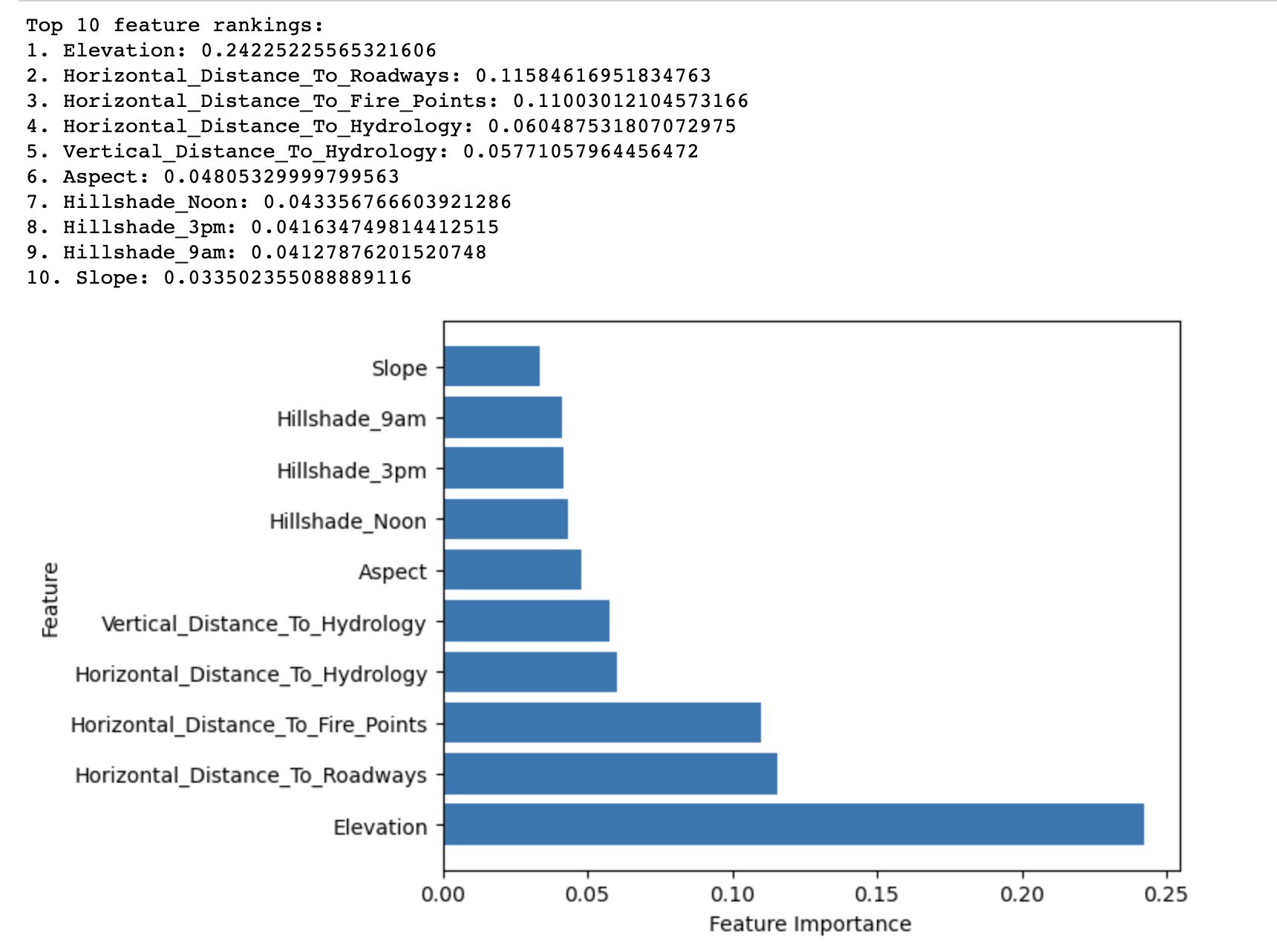
The output of the Random Forest Importance method displays the top 10 features ranked by their importance in predicting the forest cover type in the Covertype dataset.
It reveals that Elevation has the highest importance score (0.2423) among all features in predicting the forest cover type. This suggests that elevation plays a critical role in determining the dominant tree species in the Roosevelt National Forest.
Other features with relatively high importance scores include Horizontal_Distance_To_Roadways (0.1158) and Horizontal_Distance_To_Fire_Points (0.1100). These indicate that proximity to roadways and fire ignition points also significantly impacts forest cover types.
The remaining features in the top 10 list have relatively lower importance scores, but they still contribute to the overall predictive performance of the model. These features mainly relate to hydrological factors, slope, aspect, and hillshade indices.
In summary, the results highlight the most important factors affecting the distribution of forest cover types in the Roosevelt National Forest, which can be used to build a more effective and efficient predictive model for forest cover type classification.
2. Unsupervised Feature Selection Techniques
When there is no target variable available, unsupervised feature selection approaches can be used in order to reduce the dimensionality of the dataset while keeping its underlying structure. These methods often include changing the initial feature space into a new lower-dimensional space in which the changed features capture the majority of the variation in the data.
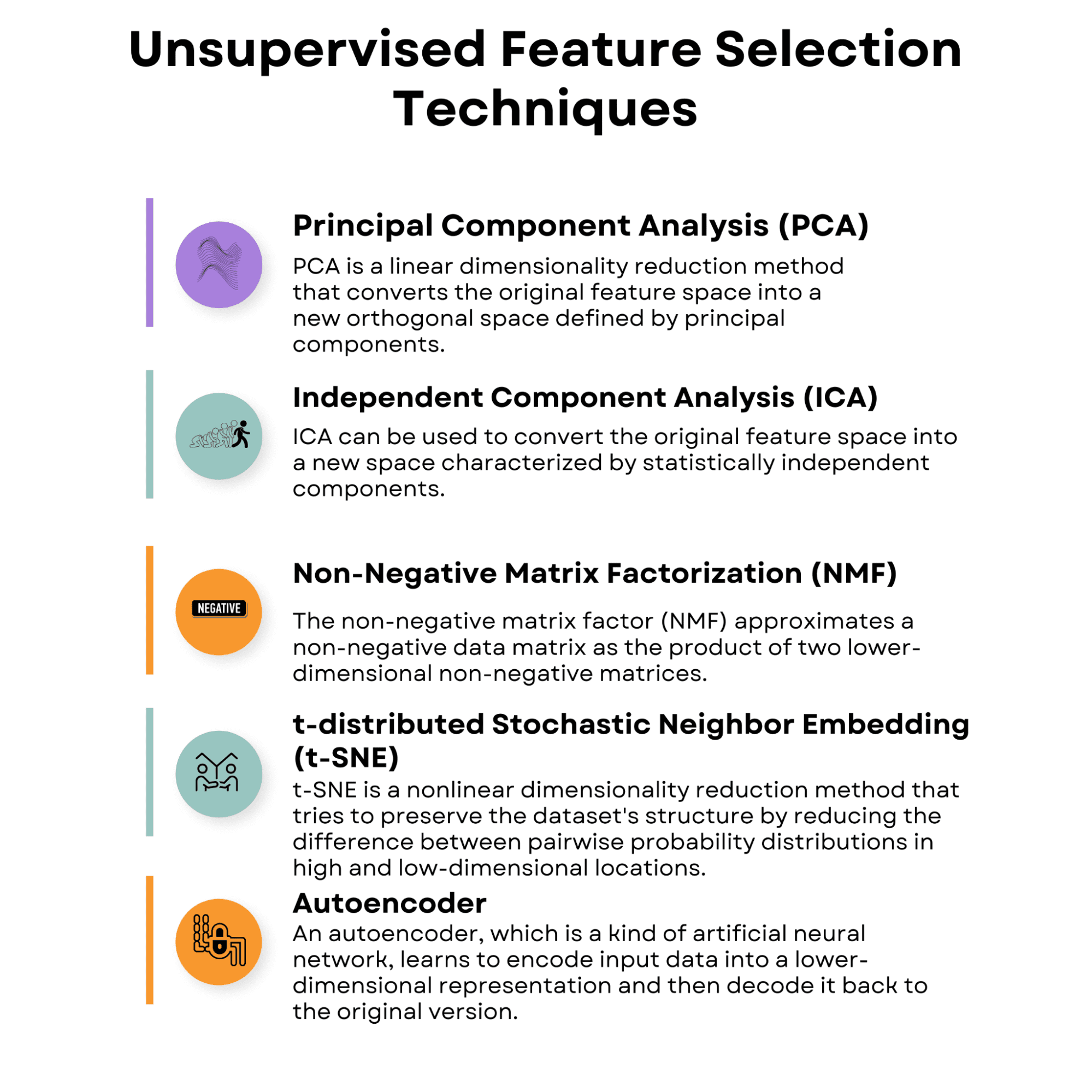
Image by Author
2.1 Principal Component Analysis (PCA)
PCA is a linear dimensionality reduction method that converts the original feature space into a new orthogonal space defined by principal components. These components are linear combinations of the original features chosen to capture the highest level of variance in the data.
PCA may be used to pick the top k principal components representing most of the variation, thus lowering the dataset's dimensionality.
To show you how this works in practice, we will work with the Wine dataset. This is a widely used dataset for classification and feature selection tasks in machine learning and consists of 178 samples, each representing a different wine originating from three different cultivars in the same region in Italy.
The goal of working with the Wine dataset is usually to build a predictive model that can accurately classify a wine sample into one of the three cultivars based on its chemical properties.
The following code demonstrates the application of Principal Component Analysis (PCA), an unsupervised feature selection technique, on the Wine dataset.
These components(principal components) capture the most variance in the data while minimizing the information loss.
The code starts by loading the Wine dataset, which consists of 13 features describing the chemical properties of different wine samples.
import numpy as np
import pandas as pd
import matplotlib.pyplot as plt
from sklearn.datasets import load_wine
from sklearn.decomposition import PCA
from sklearn.preprocessing import StandardScaler

# Load the Wine dataset
wine = load_wine()
X = wine.data
y = wine.target
feature_names = wine.feature_names
These features are then standardized using the StandardScaler to ensure that PCA is not affected by varying scales of the input features.
# Standardize the features
scaler = StandardScaler()
X_scaled = scaler.fit_transform(X)
Next, PCA is performed on the standardized data using the PCA class from the sklearn.decomposition module.
# Perform PCA
pca = PCA()
X_pca = pca.fit_transform(X_scaled)
The explained variance ratio for each principal component is calculated, indicating the proportion of the total variance in the data that each component explains.
# Calculate the explained variance ratio
explained_variance_ratio = pca.explained_variance_ratio_
Finally, two plots are generated to visualize the explained variance ratio and the cumulative explained variance by the principal components.
The first plot shows the explained variance ratio for each individual principal component, while the second plot illustrates how the cumulative explained variance increases as more principal components are included.
These plots help determine the optimal number of principal components to use in the model, balancing the trade-off between dimensionality reduction and information retention.
# Create a 2x1 grid of subplots
fig, (ax1, ax2) = plt.subplots(nrows=1, ncols=2, figsize=(16, 8))

# Plot the explained variance ratio in the first subplot
ax1.bar(range(1, len(explained_variance_ratio) + 1), explained_variance_ratio)
ax1.set_xlabel('Principal Component')
ax1.set_ylabel('Explained Variance Ratio')
ax1.set_title('Explained Variance Ratio by Principal Component')

# Calculate the cumulative explained variance
cumulative_explained_variance = np.cumsum(explained_variance_ratio)

# Plot the cumulative explained variance in the second subplot
ax2.plot(range(1, len(cumulative_explained_variance) + 1), cumulative_explained_variance, marker='o')
ax2.set_xlabel('Number of Principal Components')
ax2.set_ylabel('Cumulative Explained Variance')
ax2.set_title('Cumulative Explained Variance by Principal Components')

# Display the figure
plt.tight_layout()
plt.show()
Let’s see the whole code.
import numpy as np
import pandas as pd
import matplotlib.pyplot as plt
from sklearn.datasets import load_wine
from sklearn.decomposition import PCA
from sklearn.preprocessing import StandardScaler

# Load the Wine dataset
wine = load_wine()
X = wine.data
y = wine.target
feature_names = wine.feature_names

# Standardize the features
scaler = StandardScaler()
X_scaled = scaler.fit_transform(X)

# Perform PCA
pca = PCA()
X_pca = pca.fit_transform(X_scaled)

# Calculate the explained variance ratio
explained_variance_ratio = pca.explained_variance_ratio_

# Create a 2x1 grid of subplots
fig, (ax1, ax2) = plt.subplots(nrows=1, ncols=2, figsize=(16, 8))

# Plot the explained variance ratio in the first subplot
ax1.bar(range(1, len(explained_variance_ratio) + 1), explained_variance_ratio)
ax1.set_xlabel("Principal Component")
ax1.set_ylabel("Explained Variance Ratio")
ax1.set_title("Explained Variance Ratio by Principal Component")

# Calculate the cumulative explained variance
cumulative_explained_variance = np.cumsum(explained_variance_ratio)

# Plot the cumulative explained variance in the second subplot
ax2.plot(
    range(1, len(cumulative_explained_variance) + 1),
    cumulative_explained_variance,
    marker="o",
)
ax2.set_xlabel("Number of Principal Components")
ax2.set_ylabel("Cumulative Explained Variance")
ax2.set_title("Cumulative Explained Variance by Principal Components")

# Display the figure
plt.tight_layout()
plt.show()
Here is the output.
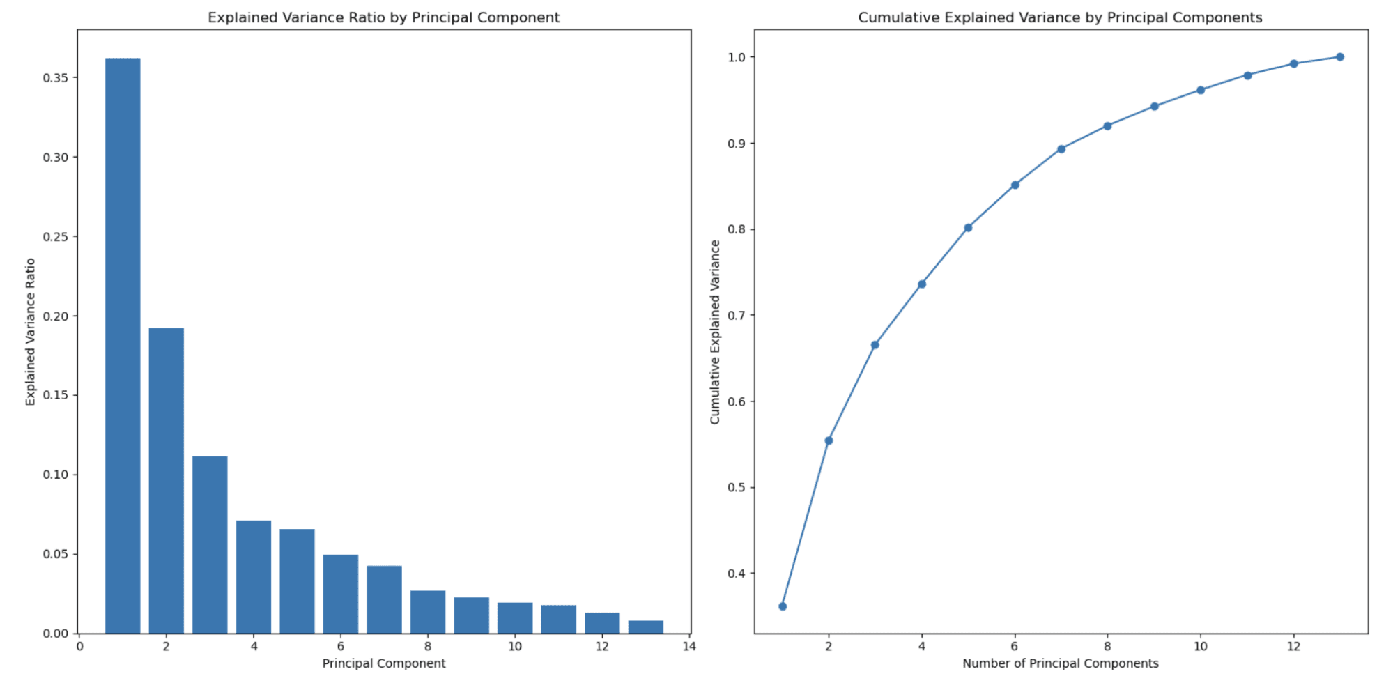
The graph on the left shows that the explained variance ratio decreases as the number of principal components increases. This is a typical behavior observed in PCA because principal components are ordered by the amount of variance they explain.
The first principal component (feature) captures the highest variance, the second principal component captures the second highest amount, and so on. As a result, the explained variance ratio decreases with each subsequent principal component.
This is one of the main reasons PCA is used for dimensionality reduction.
The second graph on the right shows the cumulative explained variance and helps you determine how many principal components (features) to select to represent the percentage of your data. The x-axis represents the number of principal components, and the y-axis shows the cumulative explained variance. As you move along the x-axis, you can see how much of the total variance is retained when you include that many principal components.
In this example, you can see that selecting around 3 or 4 principal components already captures more than 80% of the total variance, and around 8 principal components capture over 90% of the total variance.
You can choose the number of principal components based on your desired trade-off between dimensionality reduction and the variance you want to retain.
In this example, we did use Sci-kit to learn to apply PCA, and here you can find the official document.
2.2 Independent Component Analysis (ICA)
ICA is a method for dividing a multidimensional signal into its components.
In the context of feature selection, ICA can be used to convert the original feature space into a new space characterized by statistically independent components. You may decrease the dimensionality of the dataset while keeping the underlying structure by picking the top k independent components.
2.3 Non-Negative Matrix Factorization (NMF)
The non-negative matrix factor (NMF) is a dimensionality reduction approach that approximates a non-negative data matrix as the product of two lower-dimensional non-negative matrices.
NMF can be used in the context of feature selection to extract a new set of basic features that capture the important structure of the original data. You may minimize the dimensionality of the dataset while maintaining the non-negativity limitation by picking the top k basis features.
2.4 t-distributed Stochastic Neighbor Embedding (t-SNE)
t-SNE is a nonlinear dimensionality reduction method that tries to preserve the dataset's structure by reducing the difference between pairwise probability distributions in high and low-dimensional locations.
t-SNE may be applied in feature selection to project the original feature space into a lower-dimensional space that maintains the structure of the data, allowing enhanced visualization and evaluation.
You can find more information about both unsupervised algorithms and t-SNE here “Unsupervised Learning Algorithms”.
2.5 Autoencoder
An autoencoder, a kind of artificial neural network, learns to encode input data into a lower-dimensional representation and then decode it back to the original version. The autoencoder's lower-dimensional representation can be used to produce another set of features that capture the underlying structure of the original data.
Final Words
In conclusion, feature selection is vital in machine learning. It helps reduce the data's dimensionality, minimize the risk of overfitting, and improve the model's overall performance. Choosing the right feature selection method depends on the specific problem, dataset, and modeling requirements.
This article covered a wide range of feature selection techniques, including supervised and unsupervised methods.
Supervised techniques, such as filter-based, wrapper-based, and embedded approaches, use the relationship between features and the target variable to identify the most important features.
Unsupervised techniques, like PCA, ICA, NMF, t-SNE, and autoencoders, focus on the intrinsic structure of the data to reduce dimensionality without considering the target variable.
When selecting the appropriate feature selection method for your model, it's vital to consider the characteristics of your data, the underlying assumptions of each technique, and the computational complexity involved.
By carefully selecting and applying the right feature selection technique, you can significantly enhance the performance, leading to better insights and decision-making.
Nate Rosidi is a data scientist and in product strategy. He's also an adjunct professor teaching analytics, and is the founder of StrataScratch, a platform helping data scientists prepare for their interviews with real interview questions from top companies. Connect with him on Twitter: StrataScratch or LinkedIn.