Feature Selection: Where Science Meets Art
From heuristic to algorithmic feature selection techniques for data science projects.
By Mahbubul Alam, Data Scientist, Economist and Quantitative Researcher

Photo by David Clode on Unsplash
Some people say feature selection and engineering is the most important part of data science projects. In many cases it’s not sophisticated algorithms, rather it’s feature selection that makes all the difference in model performance.
Too few features can under-fit a model. For example, if you want to predict house prices, knowing just the number of bedrooms and floor area is not good enough. You are omitting many important variables a buyer cares about such as location, school district, property age etc.
You can also come from the other direction and choose 100 different features that describe every tiny detail such as names of trees on the property. Instead of adding more information, these features add noise and complexity. Many of the features chosen might be outright irrelevant. On top of that, too many features add computational costs to train a model.
So to build a good predictive model, what is the right number of features and how to choose which features to keep and which features to drop and which new features to add? This is an important consideration in machine learning projects in managing what’s known as the bias-variance tradeoff.
This is also where “science” meets “arts.”
The purpose of this article is to demystify feature selection techniques with some simple implementation. The techniques I’m describing below should equally work in regression and classification problems. Unsupervised classification (e.g. clustering) can be a bit tricky, so I’ll talk about it separately.
Heuristic approach
We don’t talk much about heuristics in data science but it is quite relevant. Let’s look at the definition (source: Wikipedia):
A heuristic or heuristic technique …. employs a practical method that is not guaranteed to be optimal, perfect, or rational, but is nevertheless sufficient for reaching an immediate, short-term goal or approximation.
This definition equally applies to feature selection, if done based on intuition. Just by looking at a dataset, you’ll get the gut feeling that such and such features are strong predictors and some others have nothing to do with the dependent variable and you feel that it’s safe to eliminate them.
If you are not sure, you can go a step further to check the correlation between features and the dependent variable.
With too many features in the dataset, just these heuristics— intuition and correlation — will get most of your job done in choosing the right features.
As an example, let’s say your company is allocating budgets for advertising in different channels (TV, radio, newspaper). You want to predict which channel is most effective as an advertisement platform and what’s the expected return.
Before you build a model you look at the historical data and found the following relationship between ad expenses on different platforms and corresponding sales revenue.
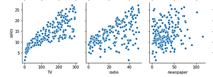
Bivariate scatterplots showing relationships between sales and ad expenditure on different platforms (figure source: author; data source: ISLR, license: GLP 2, public domain).
Based on the scatterplots what do you think are the best features to explain ad revenue? Clearly, newspaper ads do not have any significant impact on the outcome, so you may want to drop it from the model.
Automated feature selection
We will now get into automated feature selection techniques. Most of them are integrated within the sklearn module, so you can implement feature selection only in a few lines of code in a standard format.
For demonstration, I’ll use the ‘iris’ dataset (source: Kaggle/UCI Machine Learning, license: CC0 public domain). It’s a simple dataset and has only 5 columns, nevertheless, you’ll get the key points across.
Let’s load the dataset from seaborn library.
# import seaborn library
import seaborn as sns# load iris dataset
iris = sns.load_dataset('iris')
iris.head(5)

# separate features (X) from the target (y) variable
X = iris.drop('species', axis=1)
y = iris['species']
In the dataset “species” is the one that we want to predict and the remaining 4 columns are predictors. Let’s confirm the number of features programmatically:
# number of predictors in the current dataset
X.shape[1]>> 4
Let’s now go ahead and implement a few feature selection techniques.
1) Chi-squared based technique
The chi-squared-based technique selects a specific number of user-defined features (k) based on some scores. These scores are determined by computing chi-squared statistics between X (independent) and y (dependent) variables.
sklearn has built-in methods for chi-square-based feature selection. All you have to do is determine how many features you want to keep (let’s say, k=3 for the iris dataset).
# import modules
from sklearn.feature_selection import SelectKBest, chi2# select K best features
X_best = SelectKBest(chi2, k=3).fit_transform(X,y)
Let’s now confirm that we’ve got the 3 best features out of 4.
# number of best features
X_best.shape[1]>> 3
For a large number of features, you can rather specify a certain percentage of features you want to keep or drop. It works in a similar fashion as above. Let’s say we want to keep 75% of features and drop the remaining 25%.
# keep 75% top features
X_top = SelectPercentile(chi2, percentile = 75).fit_transform(X,y)# number of best features
X_top.shape[1]>> 3
2) Impurity-based feature selection
Tree-based algorithms (e.g. Random Forest Classifier) have built-in feature_importances_ attribute.
A Decision Tree would split data using a feature that decreases the impurity (measured in terms of Gini impurity or information gain). That means, finding the best feature is a key part of how the algorithm works to solve classification problems. We can then access the best features via feature_importances_ attribute.
Let’s first fit the “iris” dataset to a Random Forest Classifier with 200 estimators.
# import model
from sklearn.ensemble import RandomForestClassifier# instantiate model
model = RandomForestClassifier(n_estimators=200, random_state=0)# fit model
model.fit(X,y)
Now let’s access feature importance by the attribute call.
# importance of features in the model
importances = model.feature_importances_print(importances)>> array([0.0975945 , 0.02960937, 0.43589795, 0.43689817])
The output above shows the importance of each of the 4 features at reducing impurity at each node/split.
Since the Random Forest Classifier has many estimators (e.g. 200 decision trees above), we can calculate an estimate of the relative importance with a confidence interval. Let’s visualize it.
# calculate standard deviation of feature importances
std = np.std([i.feature_importances_ for i in model.estimators_], axis=0)# visualizationfeat_with_importance  = pd.Series(importances, X.columns)fig, ax = plt.subplots()
feat_with_importance.plot.bar(yerr=std, ax=ax)
ax.set_title("Feature importances")
ax.set_ylabel("Mean decrease in impurity")
fig.tight_layout()

Figure: Importance of features in impurity measures (source: author)
Now that we know the importance of each feature, we can manually (or visually) determine which features to keep and which one to drop.
Alternatively, we can take advantage of Scikit-Learn’s meta transformer SelectFromModel to do this job for us.
# import the transformer
from sklearn.feature_selection import SelectFromModel# instantiate and select features
selector = SelectFromModel(estimator = model, prefit=True)
X_new = selector.transform(X)
X_new.shape[1]>> 2
3) Regularization
Regularization is an important concept in machine learning to reduce overfitting (read: Avoid Overfitting with Regularization). If you have too many features, regularization controls their effect, either by shrinking feature coefficients (called L2 regularization/Ridge Regression) or by setting some feature coefficients to zero(called L1 regularization/LASSO Regression).
Some linear models have built-in L1 regularization as a hyperparameter to penalize features. Those features can be eliminated using the meta transformer SelectFromModel.
Let’s implement theLinearSVC algorithm with hyperparameter penalty = ‘l1’. We’ll then use SelectFromModelto remove some features.
# implement algorithm
from sklearn.svm import LinearSVC
model = LinearSVC(penalty= 'l1', C = 0.002, dual=False)
model.fit(X,y)# select features using the meta transformer
selector = SelectFromModel(estimator = model, prefit=True)
X_new = selector.transform(X)
X_new.shape[1]>> 2# names of selected features
feature_names = np.array(X.columns)
feature_names[selector.get_support()]>> array(['sepal_length', 'petal_length'], dtype=object)
4) Sequential selection
Sequential feature selection is an age-old statistical technique. In this case, you add (or remove) features to/from the model one by one, and check your model performance, and then heuristically choose which one to keep.
Sequential selection has two variants. The forward selection technique starts with zero feature, then adds one feature which minimizes the error the most; then adds another feature, and so on. The backward selection works in the opposite direction. The model starts with all features and calculates error; then it eliminates one feature which minimizes error even further, and so on, until the desired number of features remains.
Scikit-Learn module has SequentialFeatureSelector meta transformer to make life easier. Note that it works for sklearnv0.24 or later.
# import transformer class
from sklearn.feature_selection import SequentialFeatureSelector# instantiate model
model = RandomForestClassifier(n_estimators=200, random_state=0)# select features
selector = SequentialFeatureSelector(estimator=model, n_features_to_select=3, direction='backward')
selector.fit_transform(X,y).shape[1]>> 3# names of features selected
feature_names = np.array(X.columns)
feature_names[selector.get_support()]>> array(['sepal_width', 'petal_length', 'petal_width'], dtype=object)
Alternative techniques…
Aside from the techniques I just described, there are few other methods you can try. Some of them are not exactly designed for feature selection, but if you dig a bit deeper you will find out how they can be creatively applied for feature selection.
- Beta coefficients: the coefficients you get after running a linear regression (the beta coefficients) show the relative sensitivity of the dependent variable to each feature. From here you can choose the features with high coefficient values.
- p-value: If you implement regression in a classical statistical package (e.g.
statsmodels), you’ll notice that the model output includes p-values for each feature (check this out). The p-value tests the null hypothesis that the coefficient is exactly zero. So you can eliminate the features associated with high p-values. - Variance Inflation Factor (VIF): Typically VIF is used to detect multicollinearity in the dataset. Statisticians usually remove variables with high VIF to meet a key assumption of linear regression.
- Akaike and Bayesian Information Criteria (AIC/BIC): Generally AIC and BIC are used to compare performances between two models. But you can use it to your advantage for feature selection, for example by choosing certain features that get you a better model quality measured in terms of AIC/BIC.
- Principal Component Analysis (PCA): If you know what PCA is, you guessed it right. It’s not exactly a feature selection technique, but the dimensionality reduction properties of PCA can but used to that effect, without eliminating features entirely.
- And many others: There are quite a few other feature selection classes that come with
sklearnmodule, check out the documentation. A clustering-based algorithm has also been proposed recently in a scientific paper. Fisher’s Score is yet another technique available.
How about clustering?
Clustering is an unsupervised machine learning algorithm, meaning you feed your data into a clustering algorithm and the algorithm will figure out how to segment the data into different clusters based on some “property”. These properties actually come from the features.
Does clustering require feature selection? Of course. Without appropriate features, the clusters could be useless. Let’s say you want to segment customers in order to sell high-end, mid-range and low-end products. That means you are implicitly using customer income as a factor. You could also through education into the mix. Their age and years of experience? Sure. But as you increase the number of features, the algorithm becomes confused as to what you are trying to achieve and therefore the outputs may not be exactly what you were looking for.
All that is to say, data scientists do not run clustering algorithms in a vacuum, they often have a hypothesis or question in mind. So the features must correspond to that need.
Summary
Data scientists take feature selection very seriously because of the impact it has on model performance. For a low dimensional dataset heuristics and intuition work perfectly, however, for high dimensional data, there are automated techniques to do the job. Most useful techniques include chi-squared and impurity-based algorithms as well as regularization and sequential feature selection. In addition, there are alternative techniques that can be made useful such as beta coefficients in regression, p-value, VIF, AIC/BIC and dimensionality reduction.
In the title of this article, I said “science meets art”. It is because there’s no right or wrong answer when it comes to feature selection. We can use science tools, but in the end, it can be a subjective decision made by a data scientist.
Thanks for reading. Feel free to subscribe to be notified of my forthcoming articles or simply connect with me via Twitter or LinkedIn.
Bio: Mahbubul Alam has 8+ years of work experience applying data science in making policy and business decisions, and has worked closely with stakeholders in government and non-government organizations and helped make better decisions with data-driven solutions. Mab is passionate about statistical modeling and all aspects of data science – from survey design and data collection to building advanced predictive models. Mab is also teaching/mentoring a data science and business analytics course designed for early to mid-career analysts, team leads and IT professionals who are transitioning to data science or building data science capabilities within their organizations.
Original. Reposted with permission.
Related: