Geocoding for Data Scientists
This article introduces geocoding as part of a data science pipeline. It covers manual and API based geocoding with a fun and engaging example.
When data scientists need to know everything there is to know about the “where” of their data, they often turn to Geographic Information Systems (GIS). GIS is a complicated set of technologies and programs that serve a wide variety of purposes, but the University of Washington provides a fairly comprehensive definition, saying “a geographic information system is a complex arrangement of associated or connected things or objects, whose purpose is to communicate knowledge about features on the surface of the earth” (Lawler et al). GIS encompasses a broad range of techniques for processing spatial data from acquisition to visualization, many of which are valuable tools even if you are not a GIS specialist. This article provides a comprehensive overview of geocoding with demonstrations in Python of several practical applications. Specifically, you will determine the exact location of a pizza parlor in New York City, New York using its address and connect it to data about nearby parks. While the demonstrations use Python code, the core concepts can be applied to many programming environments to integrate geocoding into your workflow. These tools provide the basis for transforming data into spatial data and open the door for more complex geographic analysis.
What is Geocoding?
Geocoding is most commonly defined as the transformation of address data into mapping coordinates. Usually, this involves detecting a street name in an address, matching that street to the boundaries of its real-world counterpart in a database, then estimating where on the street to place the address using the street number. As an example, let’s go through the process of a simple manual geocode for the address of a pizza parlor in New York on Broadway: 2709 Broadway, New York, NY 10025. The first task is finding appropriate shapefiles for the road system of the location of your address. Note that in this case the city and state of the address are “New York, NY.” Fortunately, the city of New York publishes detailed road information on the NYC Open Data page (CSCL PUB). Second, examine the street name “Broadway.” You now know that the address can lie on any street called “Broadway” in New York city, so you can execute the following Python code to query the NYC Open Data SODA API for all streets named “Broadway.”
import geopandas as gpd
import requests
from io import BytesIO

# Request the data from the SODA API
req = requests.get(
    "https://data.cityofnewyork.us/resource/gdww-crzy.geojson?stname_lab=BROADWAY"
)
# Convert to a stream of bytes
reqstrm = BytesIO(req.content)
# Read the stream as a GeoDataFrame
ny_streets = gpd.read_file(reqstrm)
There are over 700 results of this query, but that doesn’t mean you have to check 700 streets to find your pizza. Visualizing the data, you can see that there are 3 main Broadway streets and a few smaller ones.

The reason for this is that each street is broken up into sections that correspond roughly to a block, allowing for a more granular look at the data. The next step of the process is determining exactly which of these sections the address is on using the ZIP code and street number. Each street segment in the dataset contains address ranges for the addresses of buildings on both the left and right sides of the street. Similarly, each segment contains the ZIP code for both the left and right sides of the street. To locate the correct segment, the following code applies filters to find the street segment whose ZIP code matches the address’ ZIP code and whose address range contains the street number of the address.
# Address to be geocoded
address = "2709 Broadway, New York, NY 10025"
zipcode = address.split(" ")[-1]
street_num = address.split(" ")[0]

# Find street segments whose left side address ranges contain the street number
potentials = ny_streets.loc[ny_streets["l_low_hn"] < street_num]
potentials = potentials.loc[potentials["l_high_hn"] > street_num]
# Find street segments whose zipcode matches the address'
potentials = potentials.loc[potentials["l_zip"] == zipcode]
This narrows the list to the one street segment seen below.
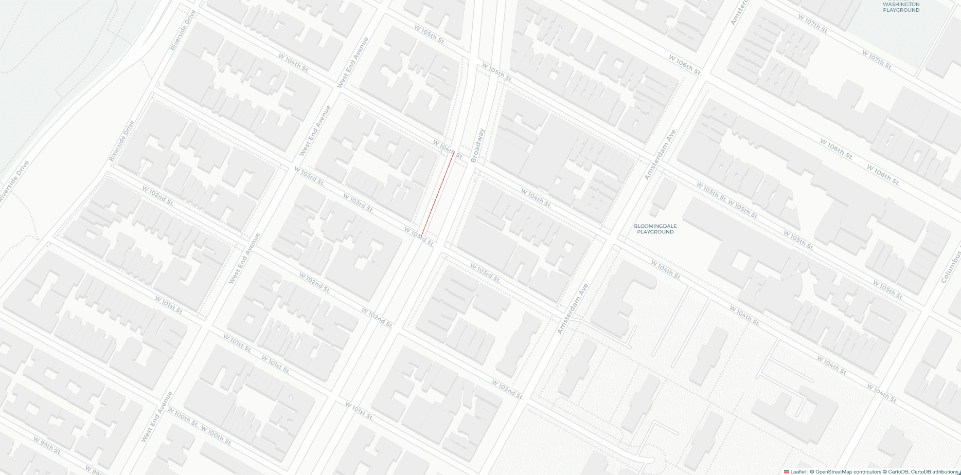
The final task is to determine where the address lies on this line. This is done by placing the street number inside the address range for the segment, normalizing to determine how far along the line the address should be, and applying that constant to the coordinates of the endpoints of the line to get the coordinates of the address. The following code outlines this process.
import numpy as np
from shapely.geometry import Point

# Calculate how far along the street to place the point
denom = (
    potentials["l_high_hn"].astype(float) - potentials["l_low_hn"].astype(float)
).values[0]
normalized_street_num = (
    float(street_num) - potentials["l_low_hn"].astype(float).values[0]
) / denom

# Define a point that far along the street
# Move the line to start at (0,0)
pizza = np.array(potentials["geometry"].values[0].coords[1]) - np.array(
    potentials["geometry"].values[0].coords[0]
)
# Multiply by normalized street number to get coordinates on line
pizza = pizza * normalized_street_num
# Add starting segment to place line back on the map
pizza = pizza + np.array(potentials["geometry"].values[0].coords[0])
# Convert to geometry array for geopandas
pizza = gpd.GeoDataFrame(
    {"address": [address], "geometry": [Point(pizza[0], pizza[1])]},
    crs=ny_streets.crs,
    geometry="geometry",
)
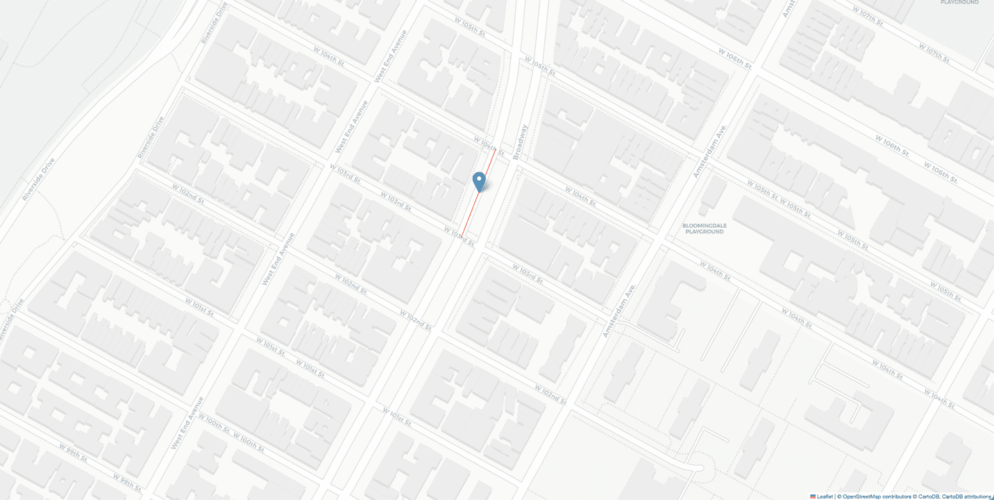
Having finished geocoding the address, it is now possible to plot the location of this pizza parlor on a map to understand its location. Since the code above looked at information pertaining to the left side of a street segment, the actual location will be slightly left of the plotted point in a building on the left side of the road. You finally know where you can get some pizza.
This process covers what is most commonly referred to as geocoding, but it is not the only way the term is used. You may also see geocoding refer to the process of transferring landmark names to coordinates, ZIP codes to coordinates, or coordinates to GIS vectors. You may even hear reverse geocoding (which will be covered later) referred to as geocoding. A more lenient definition for geocoding that encompasses these would be “the transfer between approximate, natural language descriptions of locations and geographic coordinates.” So, any time you need to move between these two kinds of data, consider geocoding as a solution.
As an alternative to repeating this process whenever you need to geocode addresses, a variety of API endpoints, such as the U.S. Census Bureau Geocoder and the Google Geocoding API, provide an accurate geocoding service for free. Some paid options, such as Esri's ArcGIS, Geocodio, and Smarty even offer rooftop accuracy for select addresses, which means that the returned coordinate lands exactly on the roof of the building instead of on a nearby street. The following sections outline how to use these services to fit geocoding into your data pipeline using the U.S. Census Bureau Geocoder as an example.
How to Geocode
In order to get the highest possible accuracy when geocoding, you should always begin by ensuring that your addresses are formatted to fit the standards of your chosen service. This will differ slightly between each service, but a common format is the USPS format of “PRIMARY# STREET, CITY, STATE, ZIP” where STATE is an abbreviation code, PRIMARY# is the street number, and all mentions of suite numbers, building numbers, and PO boxes are removed.
Once your address is formatted, you need to submit it to the API for geocoding. In the case of the U.S. Census Bureau Geocoder, you can either manually submit the address through the One Line Address Processing tab or use the provided REST API to submit the address programmatically. The U.S. Census Bureau Geocoder also allows you to geocode entire files using the batch geocoder and specify the data source using the benchmark parameter. To geocode the pizza parlor from earlier, this link can be used to pass the address to the REST API, which can be done in Python with the following code.
# Submit the address to the U.S. Census Bureau Geocoder REST API for processing
response = requests.get(
    "https://geocoding.geo.census.gov/geocoder/locations/onelineaddress?address=2709+Broadway%2C+New+York%2C+NY+10025&benchmark=Public_AR_Current&format=json"
).json()
The returned data is a JSON file, which is decoded easily into a Python dictionary. It contains a “tigerLineId” field which can be used to match the shapefile for the nearest street, a “side” field which can be used to determine which side of that street the address is on, and “fromAddress” and “toAddress” fields which contain the address range for the street segment. Most importantly, it contains a “coordinates” field that can be used to locate the address on a map. The following code extracts the coordinates from the JSON file and processes it into a GeoDataFrame to prepare it for spatial analysis.
# Extract coordinates from the JSON file
coords = response["result"]["addressMatches"][0]["coordinates"]
# Convert coordinates to a Shapely Point
coords = Point(coords["x"], coords["y"])
# Extract matched address
matched_address = response["result"]["addressMatches"][0]["matchedAddress"]
# Create a GeoDataFrame containing the results
pizza_point = gpd.GeoDataFrame(
    {"address": [matched_address], "geometry": coords},
    crs=ny_streets.crs,
    geometry="geometry",
)
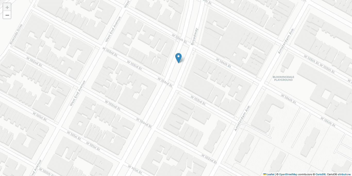
Visualizing this point shows that it is slightly off the road to the left of the point that was geocoded manually.
How to Reverse Geocode
Reverse geocoding is the process of taking geographic coordinates and matching them to natural language descriptions of a geographic region. When applied correctly, it is one of the most powerful techniques for attaching external data in the data science toolkit. The first step of reverse geocoding is determining your target geographies. This is the region that will contain your coordinate data. Some common examples are census tracts, ZIP codes, and cities. The second step is determining which, if any, of those regions the point is in. When using common regions, the U.S. Census Geocoder can be used to reverse geocode by making small changes to the REST API request. A request for determining which Census geographies contain the pizza parlor from before is linked here. The result of this query can be processed using the same methods as before. However, creatively defining the region to fit an analysis need and manually reverse geocoding to it opens up many possibilities.
To manually reverse geocode, you need to determine the location and shape of a region, then determine if the point is on the interior of that region. Determining if a point is inside a polygon is actually a fairly difficult problem, but the ray casting algorithm, where a ray starting at the point and travelling infinitely in a direction intersects the boundary of the region an odd number of times if it is inside the region and an even number of times otherwise (Shimrat), can be used to solve it in most cases. For the mathematically inclined, this is actually a direct application of the Jordan curve theorem (Hosch). As a note, if you are using data from around the world, the ray casting algorithm can actually fail since a ray will eventually wrap around the Earth’s surface and become a circle. In this case, you will instead have to find the winding number (Weisstein) for the region and the point. The point is inside the region if the winding number is not zero. Fortunately, Python’s geopandas library provides the functionality necessary to both define the interior of a polygonal region and test if a point is inside of it without all the complex mathematics.
While manual geocoding can be too complex for many applications, manual reverse geocoding can be a practical addition to your skill set since it allows you to easily match your points to highly customized regions. For example, assume you want to take your slice of pizza to a park and have a picnic. You may want to know if the pizza parlor is within a short distance of a park. New York City provides shapefiles for their parks as part of the Parks Properties dataset (NYC Parks Open Data Team), and they can also be accessed via their SODA API using the following code.
# Pull NYC park shapefiles
parks = gpd.read_file(
    BytesIO(
        requests.get(
            "https://data.cityofnewyork.us/resource/enfh-gkve.geojson?$limit=5000"
        ).content
    )
)
# Limit to parks with green area for a picnic
parks = parks.loc[
    parks["typecategory"].isin(
        [
            "Garden",
            "Nature Area",
            "Community Park",
            "Neighborhood Park",
            "Flagship Park",
        ]
    )
]
These parks can be added to the visualization to see what parks are nearby the pizza parlor.
There are clearly some options nearby, but figuring out the distance using the shapefiles and the point can be difficult and computationally expensive. Instead, reverse geocoding can be applied. The first step, as mentioned above, is determining the region you want to attach the point to. In this case, the region is “a 1/2-mile distance from a park in New York City.” The second step is calculation if the point lies inside a region, which can be done mathematically using the previously mentioned methods or by applying the “contains” function in geopandas. The following code is used to add a 1/2-mile buffer to the boundaries of the parks before testing to see which parks’ buffered regions now contain the point.
# Project the coordinates from latitude and longitude into meters for distance calculations
buffered_parks = parks.to_crs(epsg=2263)
pizza_point = pizza_point.to_crs(epsg=2263)
# Add a buffer to the regions extending the border by 1/2 mile = 2640 feet
buffered_parks = buffered_parks.buffer(2640)
# Find all parks whose buffered region contains the pizza parlor
pizza_parks = parks.loc[buffered_parks.contains(pizza_point["geometry"].values[0])]
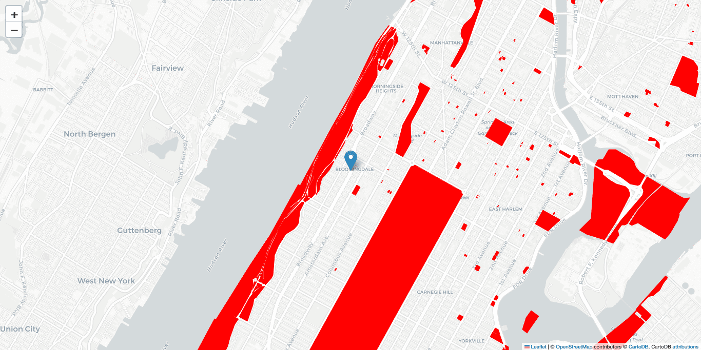
This buffer reveals the nearby parks, which are highlighted in blue in the image below

After successful reverse geocoding, you have learned that there are 8 parks within a half mile of the pizza parlor in which you could have your picnic. Enjoy that slice.

Pizza Slice by j4p4n
Sources
- Lawler, Josh and Schiess, Peter. ESRM 250: Introduction to Geographic Information Systems in Forest Resources. Definitions of GIS, 12 Feb. 2009, University of Washington, Seattle. Class Lecture. https://courses.washington.edu/gis250/lessons/introduction_gis/definitions.html
- CSCL PUB. New York OpenData. https://data.cityofnewyork.us/City-Government/road/svwp-sbcd
- U.S. Census Bureau Geocoder Documentation. August 2022. https://geocoding.geo.census.gov/geocoder/Geocoding_Services_API.pdf
- Shimrat, M., "Algorithm 112: Position of point relative to polygon" 1962, Communications of the ACM Volume 5 Issue 8, Aug. 1962. https://dl.acm.org/doi/10.1145/368637.368653
- Hosch, William L.. "Jordan curve theorem". Encyclopedia Britannica, 13 Apr. 2018, https://www.britannica.com/science/Jordan-curve-theorem
- Weisstein, Eric W. "Contour Winding Number." From MathWorld--A Wolfram Web Resource. https://mathworld.wolfram.com/ContourWindingNumber.html
- NYC Parks Open Data Team. Parks Properties. April 14, 2023. https://nycopendata.socrata.com/Recreation/Parks-Properties/enfh-gkve
- j4p4n, “Pizza Slice.” From OpenClipArt. https://openclipart.org/detail/331718/pizza-slice
Evan Miller is a Data Science Fellow at Tech Impact, where he uses data to support nonprofit and government agencies with a mission of social good. Previously, Evan used machine learning to train autonomous vehicles at Central Michigan University.